Principal Components, Dygraphs, Forecasts, Seasonal Adjustment

Example Functions, Generated by ts_. ts_prcomp calculates the principal components of multiple time series, ts_dygraphs generates an interactive graphical visualization, ts_forecast return an univariate forecast, ts_seas the seasonally adjusted series. ts_na_interpolation imputes missing values.

Usage

ts_prcomp(x, ...)

ts_dygraphs(x, ...)

ts_forecast(x, ...)

ts_seas(x, ...)

ts_na_interpolation(x, ...)

Arguments

x

ts-boxable time series, an object of class ts, xts, zoo, zooreg, data.frame, data.table, tbl, tbl_ts, tbl_time, tis, irts or timeSeries.

...

further arguments, passed to the underlying function. For help, consider these functions, e.g., stats::prcomp.

Value

a ts-boxable object of the same class as x, i.e., an object of class ts, xts, zoo, zooreg, data.frame, data.table, tbl, tbl_ts, tbl_time, tis, irts or timeSeries.

Details

With the exception of ts_prcomp, these functions depend on external packages.

See also

Vignette on how to make arbitrary functions ts-boxable.

Examples

# \donttest{
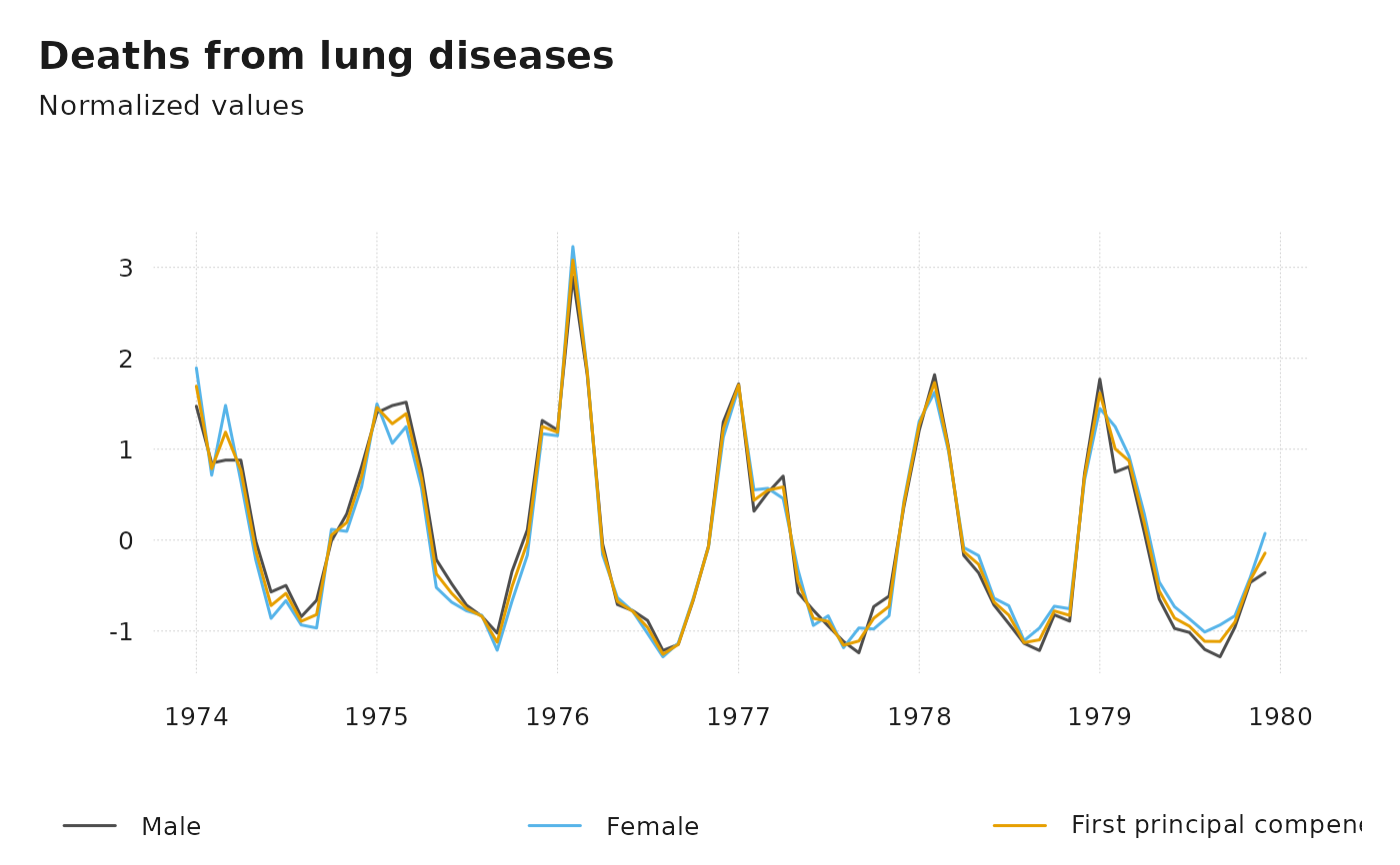
ts_plot(
  ts_scale(ts_c(
    Male = mdeaths,
    Female = fdeaths,
    `First principal compenent` = -ts_prcomp(ts_c(mdeaths, fdeaths))[, 1]
  )),
  title = "Deaths from lung diseases",
  subtitle = "Normalized values"
)


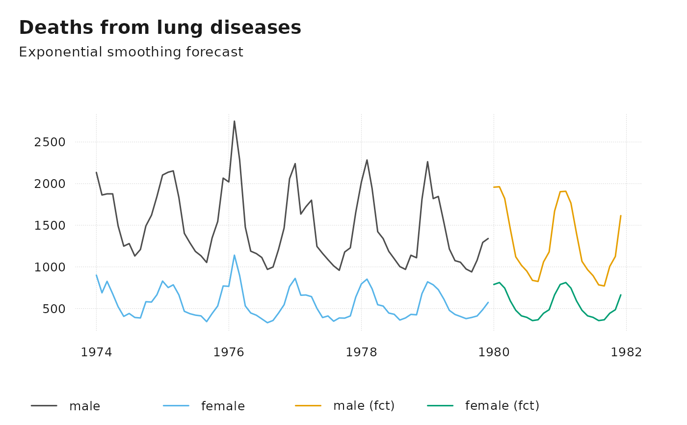
ts_plot(ts_c(
  male = mdeaths, female = fdeaths,
  ts_forecast(ts_c(`male (fct)` = mdeaths, `female (fct)` = fdeaths))
),
title = "Deaths from lung diseases",
subtitle = "Exponential smoothing forecast"
)
#> Registered S3 method overwritten by 'quantmod':
#>   method            from
#>   as.zoo.data.frame zoo 


ts_plot(
  `Raw series` = AirPassengers,
  `Adjusted series` = ts_seas(AirPassengers),
  title = "Airline passengers",
  subtitle = "X-13 seasonal adjustment"
)



# See ?imputeTS::na_interpolation for options
dta <- ts_c(mdeaths, fdeaths)
dta[c(1, 3, 10), c(1, 2)] <- NA
head(ts_na_interpolation(dta, option = "spline"))
#>           mdeaths  fdeaths
#> Jan 1974 1863.000 689.0000
#> Feb 1974 1863.000 689.0000
#> Mar 1974 1886.884 680.7926
#> Apr 1974 1877.000 677.0000
#> May 1974 1492.000 522.0000
#> Jun 1974 1249.000 406.0000

ts_dygraphs(ts_c(mdeaths, EuStockMarkets))

# }