Examples
Here you’ll find a series of example of calls to
yf_get(). Most arguments are self-explanatory, but you can
find more details at the help files.
The steps of the algorithm are:
- check cache files for existing data
- if not in cache, fetch stock prices from YF and clean up the raw data
- write cache file if not available
- calculate all returns
- build diagnostics
- return the data to the user
Fetching a single stock price
library(yfR)

# set options for algorithm
my_ticker <- 'GM'
first_date <- Sys.Date() - 30
last_date <- Sys.Date()

# fetch data
df_yf <- yf_get(tickers = my_ticker,
                first_date = first_date,
                last_date = last_date)

# output is a tibble with data
head(df_yf)
## # A tibble: 6 × 11
## ticker ref_date price_open price_high price_low price_close volume
## <chr> <date> <dbl> <dbl> <dbl> <dbl> <dbl>
## 1 GM 2026-06-01 83.4 83.4 80.4 82.7 7510600
## 2 GM 2026-06-02 82.9 84.2 81.0 81.7 10550800
## 3 GM 2026-06-03 80.7 84.1 80.3 81.7 9719500
## 4 GM 2026-06-04 82.1 83.6 81.6 83.2 6859300
## 5 GM 2026-06-05 82.0 83.1 81.4 82.1 7371600
## 6 GM 2026-06-08 81.7 84.2 81.5 83.8 8935300
## # ℹ 4 more variables: price_adjusted <dbl>, ret_adjusted_prices <dbl>,
## # ret_closing_prices <dbl>, cumret_adjusted_prices <dbl>Fetching many stock prices
library(yfR)
library(ggplot2)

my_ticker <- c('TSLA', 'GM', 'MMM')
first_date <- Sys.Date() - 100
last_date <- Sys.Date()

df_yf_multiple <- yf_get(tickers = my_ticker,
                         first_date = first_date,
                         last_date = last_date)


p <- ggplot(df_yf_multiple, aes(x = ref_date, y = price_adjusted,
                                color = ticker)) +
  geom_line()

p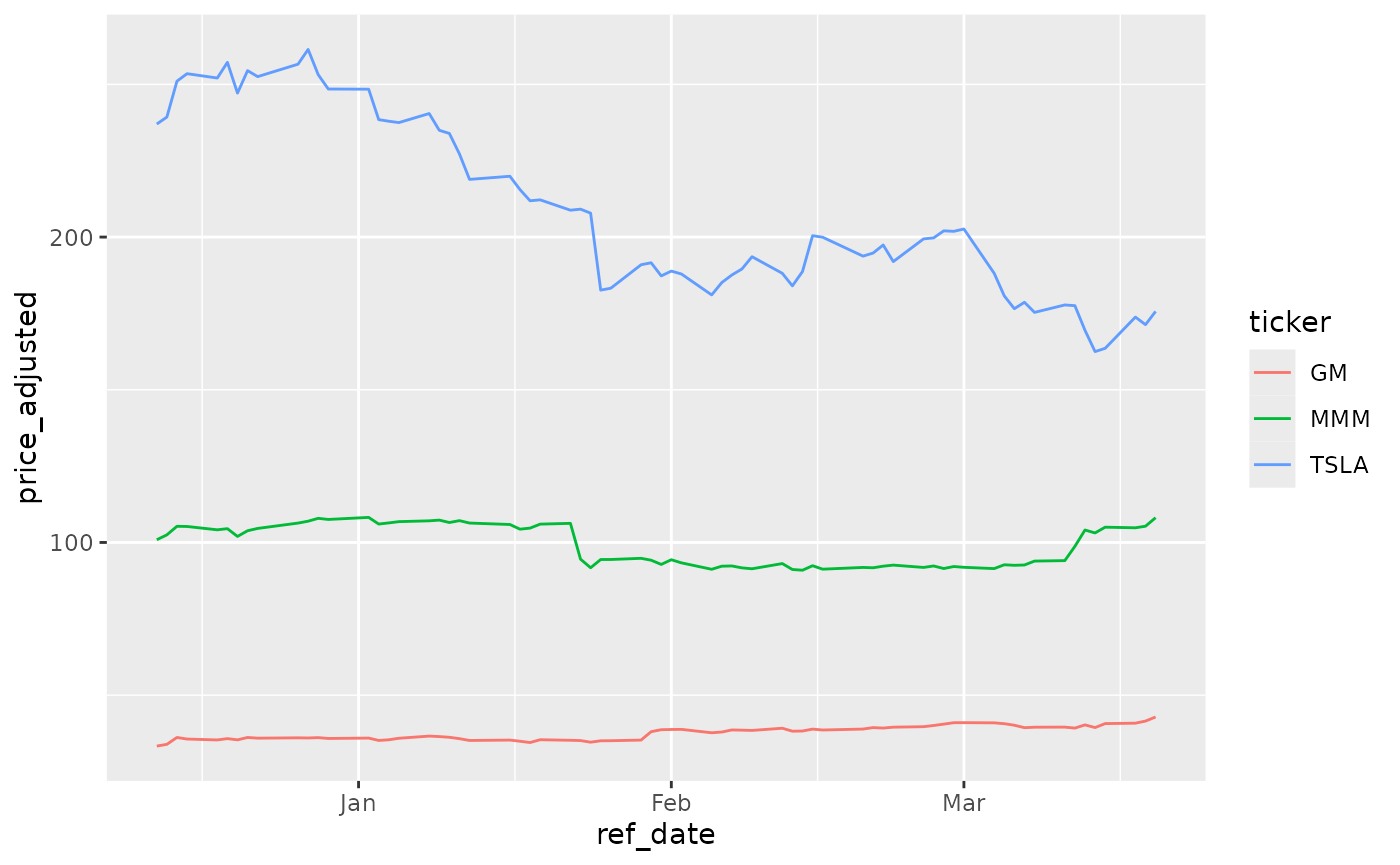
Fetching daily/weekly/monthly/yearly price data
library(yfR)
library(ggplot2)
library(dplyr)

my_ticker <- 'GE'
first_date <- '2005-01-01'
last_date <- Sys.Date()

df_dailly <- yf_get(tickers = my_ticker,
                    first_date, last_date,
                    freq_data = 'daily') %>%
  mutate(freq = 'daily')

df_weekly <- yf_get(tickers = my_ticker,
                    first_date, last_date,
                    freq_data = 'weekly') %>%
  mutate(freq = 'weekly')

df_monthly <- yf_get(tickers = my_ticker,
                     first_date, last_date,
                     freq_data = 'monthly') %>%
  mutate(freq = 'monthly')

df_yearly <- yf_get(tickers = my_ticker,
                    first_date, last_date,
                    freq_data = 'yearly') %>%
  mutate(freq = 'yearly')

# bind it all together for plotting
df_allfreq <- bind_rows(
  list(df_dailly, df_weekly, df_monthly, df_yearly)
) %>%
  mutate(freq = factor(freq,
                       levels = c('daily',
                                  'weekly',
                                  'monthly',
                                  'yearly'))) # make sure the order in plot is right

p <- ggplot(df_allfreq, aes(x = ref_date, y = price_adjusted)) +
  geom_line() +
  facet_grid(freq ~ ticker) +
  theme_minimal() +
  labs(x = '', y = 'Adjusted Prices')

print(p)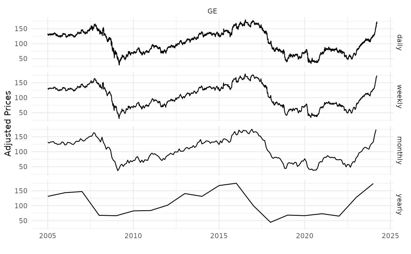
Changing format to wide
library(yfR)
library(ggplot2)

my_ticker <- c('TSLA', 'GM', 'MMM')
first_date <- Sys.Date() - 100
last_date <- Sys.Date()

df_yf_multiple <- yf_get(tickers = my_ticker,
                         first_date = first_date,
                         last_date = last_date)

print(df_yf_multiple)
## # A tibble: 207 × 11
## ticker ref_date price_open price_high price_low price_close volume
## * <chr> <date> <dbl> <dbl> <dbl> <dbl> <dbl>
## 1 GM 2026-03-23 74.8 76.8 74.6 75.7 7694800
## 2 GM 2026-03-24 75.0 76.9 74.8 76.6 7122200
## 3 GM 2026-03-25 77.9 78.3 76.4 76.6 7190700
## 4 GM 2026-03-26 76.0 77.2 74.9 75.6 8470900
## 5 GM 2026-03-27 75.2 75.3 72.7 73.0 7563200
## 6 GM 2026-03-30 73.7 74.2 72.4 72.8 7192300
## 7 GM 2026-03-31 74.1 75.1 73.4 74.5 5778200
## 8 GM 2026-04-01 75.2 75.9 74.7 75.0 5147700
## 9 GM 2026-04-02 73.3 73.7 71.7 72.5 8182800
## 10 GM 2026-04-06 72.5 73.6 72.2 73.4 5065000
## # ℹ 197 more rows
## # ℹ 4 more variables: price_adjusted <dbl>, ret_adjusted_prices <dbl>,
## # ret_closing_prices <dbl>, cumret_adjusted_prices <dbl>
l_wide <- yf_convert_to_wide(df_yf_multiple)

names(l_wide)
## [1] "price_open" "price_high" "price_low"
## [4] "price_close" "volume" "price_adjusted"
## [7] "ret_adjusted_prices" "ret_closing_prices" "cumret_adjusted_prices"
prices_wide <- l_wide$price_adjusted
head(prices_wide)
## # A tibble: 6 × 4
## ref_date GM MMM TSLA
## <date> <dbl> <dbl> <dbl>
## 1 2026-03-23 75.6 146. 381.
## 2 2026-03-24 76.4 146. 383.
## 3 2026-03-25 76.4 147. 386.
## 4 2026-03-26 75.4 143. 372.
## 5 2026-03-27 72.8 142. 362.
## 6 2026-03-30 72.6 142. 355.