eLTER_eu_networks <- readr::read_csv("./data/eLTER_eu_networks.csv", show_col_types = FALSE) %>%
  tibble::as_tibble()

related_resources <- purrr::map_dfr(
  as.list(
    eLTER_eu_networks$DEIMS.iD
  ),
  function (x) {
    part <- ReLTER::get_network_related_resources(x)
    if(!is.null(part)) part %>%
      dplyr::filter(!is.na(uri)) %>%
      dplyr::mutate(
        networkID = x,
        type = stringr::str_replace(uri, "https://deims.org/(.*)/.*","\\1")
      )
  }
) %>%
  dplyr::inner_join(eLTER_eu_networks, by = c("networkID" = "DEIMS.iD")) %>%
  dplyr::select(
    title = relatedResourcesTitle,
    uri,
    lastChanged = relatedResourcesChanged,
    networkID,
    type,
    network = eLTER_EU_Networks,
    country
  )
library(dplyr)
tbl_resources <- related_resources %>%
  dplyr::count(country, type) %>%
  tidyr::pivot_wider(names_from = type, values_from = n, values_fill = 0)

knitr::kable(
  tbl_resources,
  caption = "eLTER EU networks related resources"
)
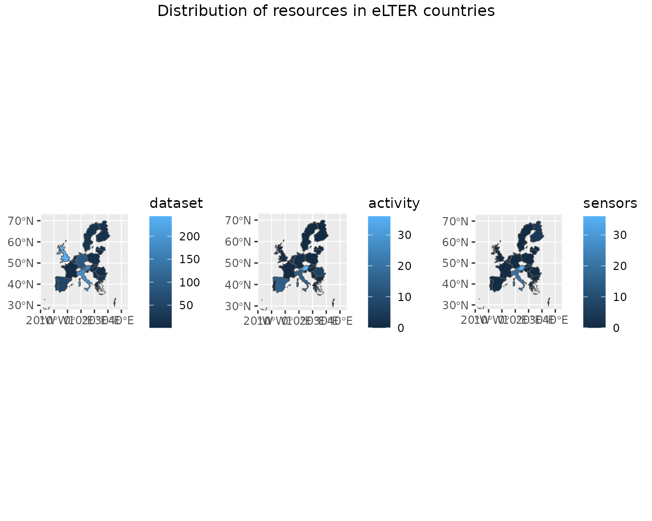
eLTER EU networks related resources
| Austria |
36 |
165 |
36 |
| Belgium |
1 |
7 |
0 |
| Bulgaria |
0 |
15 |
0 |
| Finland |
0 |
16 |
4 |
| France |
0 |
2 |
0 |
| Germany |
1 |
89 |
0 |
| Greece |
0 |
3 |
0 |
| Hungary |
0 |
17 |
0 |
| Israel |
0 |
18 |
0 |
| Italy |
15 |
190 |
20 |
| Latvia |
0 |
14 |
0 |
| Lithuania |
0 |
2 |
0 |
| Netherlands |
0 |
2 |
0 |
| Poland |
0 |
11 |
0 |
| Portugal |
0 |
44 |
0 |
| Romania |
7 |
8 |
0 |
| Serbia |
0 |
1 |
0 |
| Slovakia |
0 |
6 |
0 |
| Slovenia |
0 |
3 |
0 |
| Spain |
15 |
53 |
0 |
| Sweden |
0 |
21 |
0 |
| United Kingdom |
0 |
243 |
0 |
# Get the world map
worldMap <- rworldmap::getMap()

library(rnaturalearth)
world_map <- rnaturalearth::ne_countries(scale = 50, returnclass = 'sf')
europe_map <- world_map %>%
  filter(name %in% related_resources$country)

elter_map <- europe_map %>%
  dplyr::select(
    name,
    geometry
  ) %>%
  dplyr::left_join(tbl_resources, by = c("name" = "country"))

map_datasets <- ggplot2::ggplot() +
  ggplot2::geom_sf(data = elter_map, ggplot2::aes(fill = dataset)) +
  ggplot2::coord_sf(xlim = c(-20, 45), ylim = c(28, 73), expand = FALSE)
map_activities <- ggplot2::ggplot() +
  ggplot2::geom_sf(data = elter_map, ggplot2::aes(fill = activity)) +
  ggplot2::coord_sf(xlim = c(-20, 45), ylim = c(28, 73), expand = FALSE)
map_sensors <- ggplot2::ggplot() +
  ggplot2::geom_sf(data = elter_map, ggplot2::aes(fill = sensors)) +
  ggplot2::coord_sf(xlim = c(-20, 45), ylim = c(28, 73), expand = FALSE)

gridExtra::grid.arrange(
  map_datasets,
  map_activities,
  map_sensors,
  nrow = 1,
  top = "Distribution of resources in eLTER countries"#,
  # bottom = grid::textGrob(
  #   "this footnote is right-justified",
  #   gp = grid::gpar(fontface = 3, fontsize = 9),
  #   hjust = 1,
  #   x = 1
  # )
)
## Warning: Using `size` aesthetic for lines was deprecated in ggplot2 3.4.0.
## ℹ Please use `linewidth` instead.