fellingdater: Estimate, report and combine felling
dates of historical tree-ring series
This R-package offers a suite of functions designed to assist you in inferring estimates for felling dates from dated tree-ring series. The presence of (partially) preserved sapwood or waney edge allows on a (pre-)historical timber allows to estimate the missing number of sapwood rings. from this estimate, a range for the actual felling date can be determined and reported, for individual series as well as for a group of related timbers.
In cases where it can be assumed that a group of historical timbers were all felled simultaneously (i.e., in the same year), but due to the absence of the bark/cambial zone (waney edge) and the final formed tree ring, this cannot be determined, the preserved sapwood rings can be used to establish a date range for the felling event.
Taking into account the observed number of sapwood rings across all analysed samples and combining them into a single estimate, a more accurate and precise estimation of the felling date year for the group of timbers under study is likely to be obtained.
This vignette provides a quick overview of the package main functions, including a new tool to sum sapwood probability distributions, comparable to ‘summed probability densities (SPD)’ commonly applied to sets of radiocarbon (14C) dates.
Installation
The latest developing version is hosted on GitHub and R-universe, and can be installed locally:
# install.packages("pak")
pak::pak("ropensci/fellingdater")
or
install.packages("fellingdater", repos = "https://ropensci.r-universe.dev")Basic example
In the following example the combined felling date range for a set of five dated tree-ring series is computed:
## a data set where all series have partially preserved sapwood:
sw_combine(sw_example1, plot = TRUE)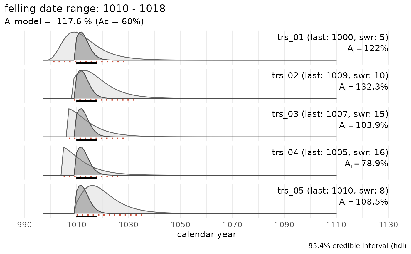
The light grey distributions represent the probability density function of the felling date range for each individual series. The dark grey distribution is the combined estimate for a common felling date.
The sapwood data used in the example above to estimate the felling date range, was published by Hollstein (1980) :
sw_model("Hollstein_1980", plot = TRUE)
Main functions
sw_interval
This function calculates the probability density function (PDF) and the highest probability density interval (HDI) for the range of potential felling dates, based on the observed number of sapwood rings, their chronological dating and the selected sapwood data and model.
In the example below, we observe 10 sapwood rings on a sample (with the last ring dated to 1234 AD) that originates from the Southern Baltic region. The sapwood model published by Wazny, 1990 covers this provenance region. The hdi delineates an interval in which the actual felling date is most likely situated. It represents the shortest interval within a probability distribution for a given probability mass or credible interval. The HDI summarizes the distribution by specifying an interval that spans most of the distribution, typically 95%, such that every point inside the interval has higher credibility than any point outside the interval.
sw_interval(
     n_sapwood = 10,
     last = 1234,
     hdi = TRUE,
     cred_mass = .95,
     sw_data = "Wazny_1990",
     densfun = "lognormal"
)
#>   lower upper         p
#> 1  1234  1250 0.9611793
When hdi = FALSE, a matrix is returned with scaled
p-values for each number of observed sapwood rings.
The results of this procedure can be visualized by setting
plot = TRUE.
# 10 sapwood rings observed and the Wazny 1990 sapwood model:
sw_interval(
     n_sapwood = 10,
     last = 1234,
     hdi = TRUE,
     cred_mass = .95,
     sw_data = "Wazny_1990",
     densfun = "lognormal",
     plot = TRUE
)
fd_report
The fd_report()function reports estimates of the felling
date (fd) range for individual series.
tmp <- data.frame(
     id = c("aaa", "bbb", "ccc"),
     swr = c(10, 11, 12),
     waneyedge = c(FALSE, FALSE, TRUE),
     end = c(123, 456, 1789)
)
fd_report(tmp,
     series = "id",
     n_sapwood = "swr",
     last = "end",
     sw_data = "Wazny_1990"
)
#>   series last n_sapwood waneyedge lower upper        felling_date sapwood_model
#> 1    aaa  123        10     FALSE   123   139 between 123 and 139    Wazny_1990
#> 2    bbb  456        11     FALSE   456   471 between 456 and 471    Wazny_1990
#> 3    ccc 1789        12      TRUE    NA  1789             in 1789    Wazny_1990
sw_combine
The the sw_combine() function combines felling dates of
a group of related series with (partially) preserved sapwood, in order
to narrow down the range of a common felling date. The function returns
a list with:
the PDF for the felling date of the individual series and the PDF of the model that combines these individual series (
$dataRaw),the HDI for the combined estimate of the common felling date (
$hdi_model),the Agreement index (
$A_comb) of the model, expressing how well the individual series fit into the model (ideally around 100%, and not lower than the critical threshold A_c = 60%) ,an overview of the felling date range for the individual series (
$individual_series), and their Agreement index (A_i) to the combined model.
sw_example0
A data set with dated tree-ring series, all with partially preserved
sapwood. The names of the variables in the data set are mapped to the
parameters of the sw_combine() function. In the example
below, the numeric output is returned:
sw_example0
#>      trs  end swr  bark
#> 1 trs_01 1000   5 FALSE
#> 2 trs_02 1009  10 FALSE
#> 3 trs_03 1007  15 FALSE
#> 4 trs_04 1005  16 FALSE
#> 5 trs_05 1010   8 FALSE
# In sw_example0, the column names are not equivalent to the default names in `sw_combine()`.

output_comb <- sw_combine(sw_example0,
     series = "trs",
     last = "end",
     n_sapwood = "swr",
     waneyedge = "bark",
     cred_mass = .954,
     plot = FALSE
)

head(output_comb$rawData, 20)
#> NULL

output_comb[-1]
#> $sapwood_data
#> [1] "Hollstein_1980"
#>
#> $sapwood_model
#> [1] "lognormal"
#>
#> $cred_mass
#> [1] 0.954
#>
#> $hdi_model
#>   lower upper         p
#> 1     6    34 0.9561277
#>
#> $hdi_combine
#>   lower upper         p
#> 1  1010  1018 0.9741642
#>
#> $individual_series
#>   series last n_sapwood waneyedge lower upper agr_index
#> 1 trs_01 1000         5     FALSE  1001  1029     122.0
#> 2 trs_02 1009        10     FALSE  1009  1033     132.3
#> 3 trs_03 1007        15     FALSE  1007  1029     103.9
#> 4 trs_04 1005        16     FALSE  1005  1026      78.9
#> 5 trs_05 1010         8     FALSE  1010  1036     108.5
#>
#> $A_model
#> Overall agreement index (%)
#>                       117.6
#>
#> $A_c
#> Critical threshold (%)
#>                     60
#>
#> $model_summary
#> [1] "felling date range:  1010  -  1018"
sw_example2
A data set with 5 tree-ring series, one of which has an exact felling date (waney edge present):
sw_example2
#>   series last n_sapwood waneyedge
#> 1 trs_06 1000         5     FALSE
#> 2 trs_07 1005        10     FALSE
#> 3 trs_08 1008        NA     FALSE
#> 4 trs_09 1000         1     FALSE
#> 5 trs_10 1010        15      TRUE

sw_combine(sw_example2, plot = TRUE)
sw_example3
A data set where all tree-ring series have been measured up to the waney edge:
sw_combine(sw_example3, plot = TRUE)
sw_example4
An attempt to compute a common felling date for a group of tree-ring series, all including partially preserved sapwood:
sw_combine(sw_example4, plot = TRUE)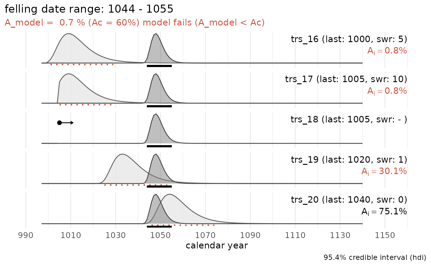
No common felling date can be computed for this particular data set. The model fails (agreement index of the model is below the critical threshold value (A_c) of 60%). Three series have an individual agreement index below 60%.
sw_example5
When no sapwood rings are observed and measured, only an
earliest possible felling date (terminus post
quem) can be determined:
sw_combine(sw_example5, plot = TRUE)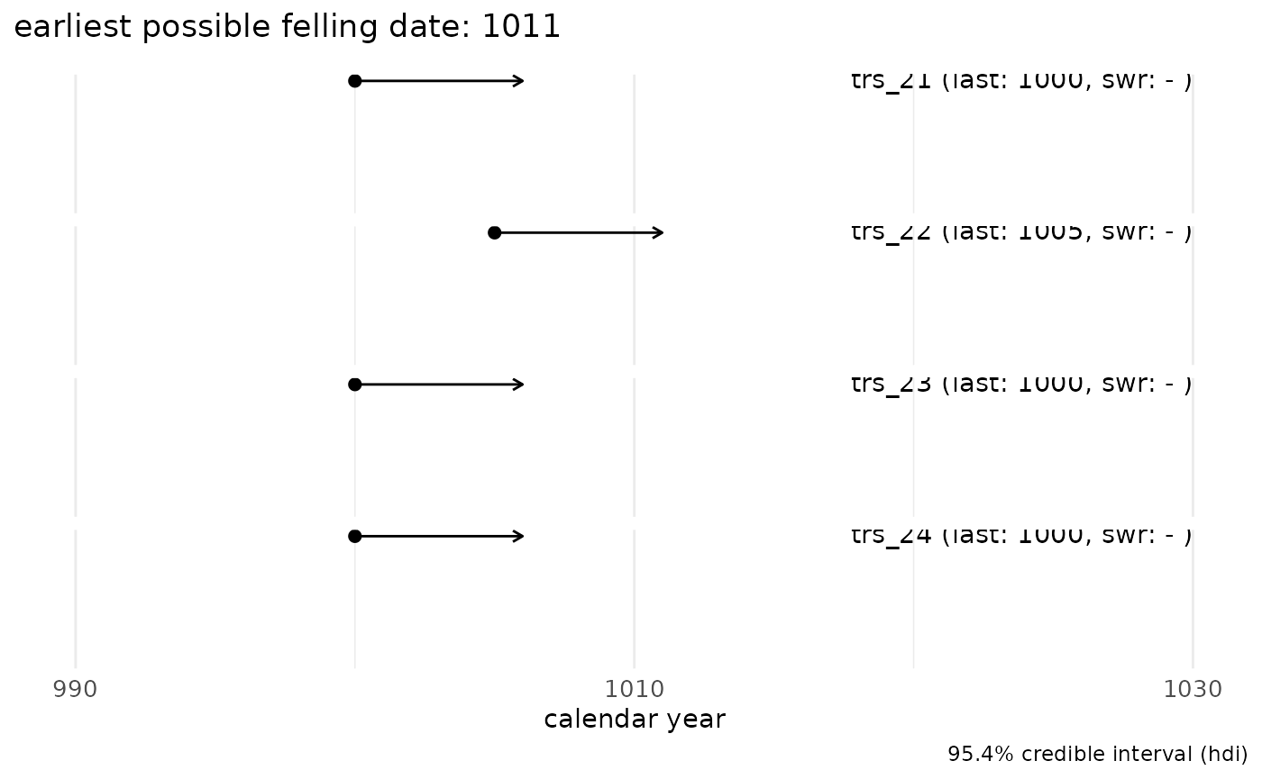
sw_sum
The sw_sum() function calculates the the summed
probability density (SPD) for a set of felling date ranges. In the
example, the SPD for a set of 9 series with partially preserved sapwood
or waney edge is computed and plotted. A smoother for the SPD is plotted
as well. The dots represent exact felling dates (i.e., series with waney
edge).
spd7 <- sw_sum(sw_example7, plot = FALSE)
#> --> 1 series without sapwood rings or waney edge detected
#>         and removed from the data set
sw_sum_plot(spd7, window_smooth = 5, bar_col = "#95d5b2", trend_col = "#dda15e", dot_col = "forestgreen", dot_shape = 23, dot_size = 4)
Helper functions
sw_data_overview
The function sw_data_overview() provides an overview of
all published sapwood data sets distributed with this package.
sw_data_overview()
#>  [1] "Brathen_1982"     "Hollstein_1980"   "Miles_1997_NM"    "Miles_1997_SC"
#>  [5] "Miles_1997_WBC"   "Pilcher_1987"     "Sohar_2012_ELL_c" "Sohar_2012_ELL_t"
#>  [9] "Sohar_2012_FWE_c" "Sohar_2012_FWE_t" "vanDaalen_NLBE"   "vanDaalen_Norway"
#> [13] "Wazny_1990"       "Weitz_2025"
Load the original data with, for example,
get("Hollstein_1980").
sw_data_info
More information on one of the sapwood data sets - how to cite the
data set, the geographical area the data represents, the number of
observations and some basic summary stats - can be retrieved by using
the sw_data_info() function.
sw_data_info("Pilcher_1987")
#> $data
#> [1] "Pilcher_1987"
#>
#> $citation
#> [1] "Pilcher J.R. 1987. A 700 year dating chronology for northern France. Applications of tree-ring studies. Current research in dendrochronology and related subjects. BAR International Series 333, 127–139."
#>
#> $area
#> [1] "Northern France"
#>
#> $n_observations
#> [1] 116
#>
#> $summary_raw_data
#>    Min. 1st Qu.  Median    Mean 3rd Qu.    Max.
#>   12.00   22.00   26.00   26.72   31.00   49.00
sw_model and sw_model_plot()
A graphical representation of a sapwood data set is provided by the
sw_model_plot() function.
tmp <- sw_model(
     sw_data = "Sohar_2012_ELL_c",
     densfun = "lognormal",
     cred_mass = 0.95,
     plot = FALSE
)

sw_model_plot(tmp,
     bar_fill = "steelblue3",
     bar_color = "grey60",
     line_color = "red3"
)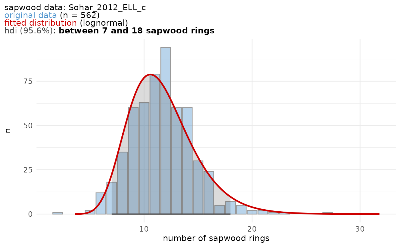
sw_data_info("Sohar_2012_ELL_c")
#> $data
#> [1] "Sohar_2012_ELL_c"
#>
#> $citation
#> [1] "Sohar K., Vitas A. & Läänelaid A. 2012. Sapwood estimates of pedunculate oak (Quercus robur L.) in eastern Baltic, Dendrochronologia 30.1, 49–56. DOI: https://doi.org/10.1016/j.dendro.2011.08.001"
#>
#> $area
#> [1] "Eastern Estonia, Latvia, Lithuania (sapwood determined by color)."
#>
#> $n_observations
#> [1] 562
#>
#> $summary_raw_data
#>    Min. 1st Qu.  Median    Mean 3rd Qu.    Max.
#>    2.00   10.00   12.00   11.69   13.00   27.00
The sw_model() function fits a distribution to a data
set of observed sapwood numbers and computes the highest posterior
density interval (HDI) for a given credibility mass. The density
function fitted to the sapwood data set should be one of:
- “lognormal” (the default value),
- “normal”,
- “weibull”,
- “gamma”.
The credible interval should be a value between 0 and 1.
sw_model("Wazny_1990", densfun = "gamma", cred_mass = .90, plot = TRUE)
#> Warning in densfun(x, parm[1], parm[2], ...): NaNs produced
When plot = FALSE, a list with the numeric output of the
modelling process is returned.
read_fh and get_header
The read_fh() function is an extension to the
dplR::read.fh() function from the dplR
package (Bunn 2008, Bunn 2010, Bunn et al. 2022).
It allows to read .fh (format Heidelberg) files of ring widths AND
additional information found in the HEADER fields are listed as
attributes.
This function also works with ring-width data in CHRONO and HALF-CHRONO format.
Furthermore, the read_fh() function is case
insensitive.
In the example below, an .fh file with dated tree-ring series from a
medieval ship DOEL1 is read with read_fh(). The ring width
measurement, in different formats, are converted to a
data.frame.
Doel1 <- system.file("extdata", "DOEL1.fh", package = "fellingdater")

Doel1_trs <- read_fh(Doel1, verbose = FALSE)

head(Doel1_trs, 15)
#>      K1_091 S38-BB GD3-1BB GR1mBB GQ1mBB K1_095 GG1-1BB S13mSB S13A-BB S6-SB
#> 1150     NA     NA      NA     NA   3.80     NA      NA     NA      NA    NA
#> 1151     NA     NA      NA     NA   4.15     NA      NA     NA      NA    NA
#> 1152     NA     NA      NA     NA   4.63     NA      NA     NA      NA    NA
#> 1153     NA     NA      NA     NA   4.31     NA      NA     NA      NA    NA
#> 1154     NA     NA      NA     NA   3.97     NA      NA     NA      NA    NA
#> 1155     NA     NA      NA     NA   4.10     NA      NA     NA      NA    NA
#> 1156     NA     NA      NA     NA   2.02     NA      NA     NA      NA    NA
#> 1157     NA     NA      NA     NA   3.24     NA      NA     NA      NA    NA
#> 1158   2.50     NA      NA     NA   3.75     NA      NA     NA      NA    NA
#> 1159   2.73     NA      NA     NA   3.07     NA      NA     NA      NA    NA
#> 1160   2.27     NA      NA     NA   4.19     NA      NA     NA      NA    NA
#> 1161   1.44     NA      NA     NA   3.74     NA      NA     NA      NA    NA
#> 1162   1.47     NA      NA     NA   4.54     NA      NA     NA      NA    NA
#> 1163   2.29     NA      NA     NA   4.61     NA      NA     NA      NA    NA
#> 1164   2.83     NA      NA     NA   3.91     NA      NA   1.84      NA    NA
When header = TRUE, the get_header()
function is triggered and HEADER fields in the .fh file are returned as
a data.frame, instead of the ring-width measurements.
read_fh(Doel1, verbose = FALSE, header = TRUE)
#>     series data_type         chrono_members species first last length n_sapwood
#> 1   K1_091    Single                   <NA>    QUSP  1158 1292    135        15
#> 2   S38-BB    Single                   <NA>    QUSP  1193 1306    114         0
#> 3  GD3-1BB    Single                   <NA>    QUSP  1222 1310     89         5
#> 4   GR1mBB    Quadro K1_001,K1_004x,GR1-3BB    QUSP  1220 1310     91         3
#> 5   GQ1mBB    Quadro  GQ1-2BB,K1_007,K1_009    QUSP  1150 1314    165         7
#> 6   K1_095    Single                   <NA>    QUSP  1207 1320    114        21
#> 7  GG1-1BB    Single                   <NA>    QUSP  1240 1322     83        13
#> 8   S13mSB    Quadro          S1-3SB,K1_076    QUSP  1164 1322    159        20
#> 9  S13A-BB    Single                   <NA>    QUSP  1232 1324     93        19
#> 10   S6-SB    Single                   <NA>    QUSP  1221 1324    104        14
#>    n_sapwood_chr unmeasured_rings invalid_rings status waneyedge bark pith
#> 1           <NA>               NA            NA  Dated      <NA> <NA>    -
#> 2           <NA>               NA            NA  Dated      <NA> <NA>    -
#> 3           <NA>               NA            NA  Dated      <NA> <NA>    -
#> 4           <NA>               NA            NA  Dated       ---    -    -
#> 5           <NA>               NA            NA  Dated       ---    -    -
#> 6           <NA>               NA            NA  Dated      <NA>    -    -
#> 7           <NA>               NA            NA  Dated      <NA> <NA> <NA>
#> 8           <NA>               NA            NA  Dated       --- <NA>    -
#> 9           <NA>               NA             1  Dated       WKE <NA> <NA>
#> 10          <NA>               NA             1  Dated       WKE <NA> <NA>
#>    pith_offset pith_offset_delta                                  comments
#> 1           NA                NA                                 keelplank
#> 2           NA                NA  HW/SW boundary | K1_281 | framing timber
#> 3           NA                NA                       K1_370 | hull plank
#> 4           NA                NA                                hull plank
#> 5           NA                NA                                hull plank
#> 6           NA                NA                                inner stem
#> 7           NA                NA                                hull plank
#> 8           NA                NA average of S1-3SB,K1_076 | framing timber
#> 9           NA                NA                            framing timber
#> 10          NA                NA                            framing timber
#>                project                location town  zip       street
#> 1  Ship timbers DOEL 1       Doel_Deurganckdok <NA> <NA>         <NA>
#> 2  Ship timbers DOEL 1       Doel_Deurganckdok <NA> <NA>         <NA>
#> 3  Ship timbers DOEL 1       Doel_Deurganckdok <NA> <NA>         <NA>
#> 4  Ship timbers DOEL 1       Doel_Deurganckdok Doel <NA> Deurganckdok
#> 5  Ship timbers DOEL 1       Doel_Deurganckdok Doel <NA> Deurganckdok
#> 6  Ship timbers DOEL 1       Doel_Deurganckdok Doel <NA> Deurganckdok
#> 7                 <NA> KOGGE ANTWERPEN GG1-1BB <NA> <NA>         <NA>
#> 8  Ship timbers DOEL 1       Doel_Deurganckdok <NA> <NA>         <NA>
#> 9  Ship timbers DOEL 1       Doel_Deurganckdok <NA> <NA>         <NA>
#> 10                <NA>   KOGGE ANTWERPEN S6-SB <NA> <NA>         <NA>
#>    sampling_date measuring_date personal_id client_id longitude  latitude
#> 1           <NA>           <NA>          KH      <NA>  4.269711 51.298236
#> 2           <NA>           <NA>          KH      <NA>  4.269711 51.298236
#> 3           <NA>           <NA>          KH      <NA>  4.269711 51.298236
#> 4           <NA>           <NA>          KH      <NA>  4.269711 51.298236
#> 5           <NA>           <NA>          KH      <NA>  4.269711 51.298236
#> 6           <NA>           <NA>          KH      <NA>  4.269711 51.298236
#> 7           <NA>           <NA>        <NA>      <NA>  4.269711 51.298236
#> 8           <NA>           <NA>          KH      <NA>  4.269711 51.298236
#> 9           <NA>           <NA>        <NA>      <NA>  4.269711 51.298236
#> 10          <NA>           <NA>        <NA>      <NA>  4.269711 51.298236
The data.frame with the HEADER fields can then be used
as input for the sw_functions:
Doel1_header <- read_fh(Doel1, verbose = FALSE, header = TRUE)

Doel1_header |>
     # first convert column 'waneyedge' to a logical vector
     # (in the original .fh file header fields the presence of waney edge is
     # indicated by "WK" - a character string - in the corresponding HEADER field)
     dplyr::mutate(waneyedge = dplyr::if_else(grepl("wk", waneyedge, ignore.case = TRUE),
          TRUE, FALSE
     )) |>
     sw_combine(plot = TRUE)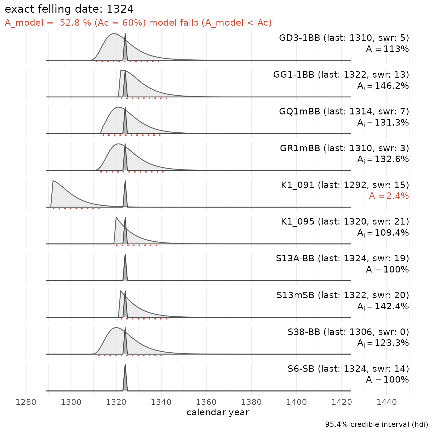
The attempt to combine the dated tree-ring series from DOEL1 into a single felling-date range fails. These tree-ring series cannot represent a single event.
However, leaving out the tree-ring series of the keelplank (series “K1_091”) of this medieval ship shows that the hull planking and some frame elements could share a common felling date:
Doel1_header |>
     dplyr::mutate(waneyedge = dplyr::if_else(grepl("wk", waneyedge, ignore.case = TRUE),
          TRUE, FALSE
     )) |>
     dplyr::filter(series != "K1_091") |>
     sw_combine(plot = TRUE)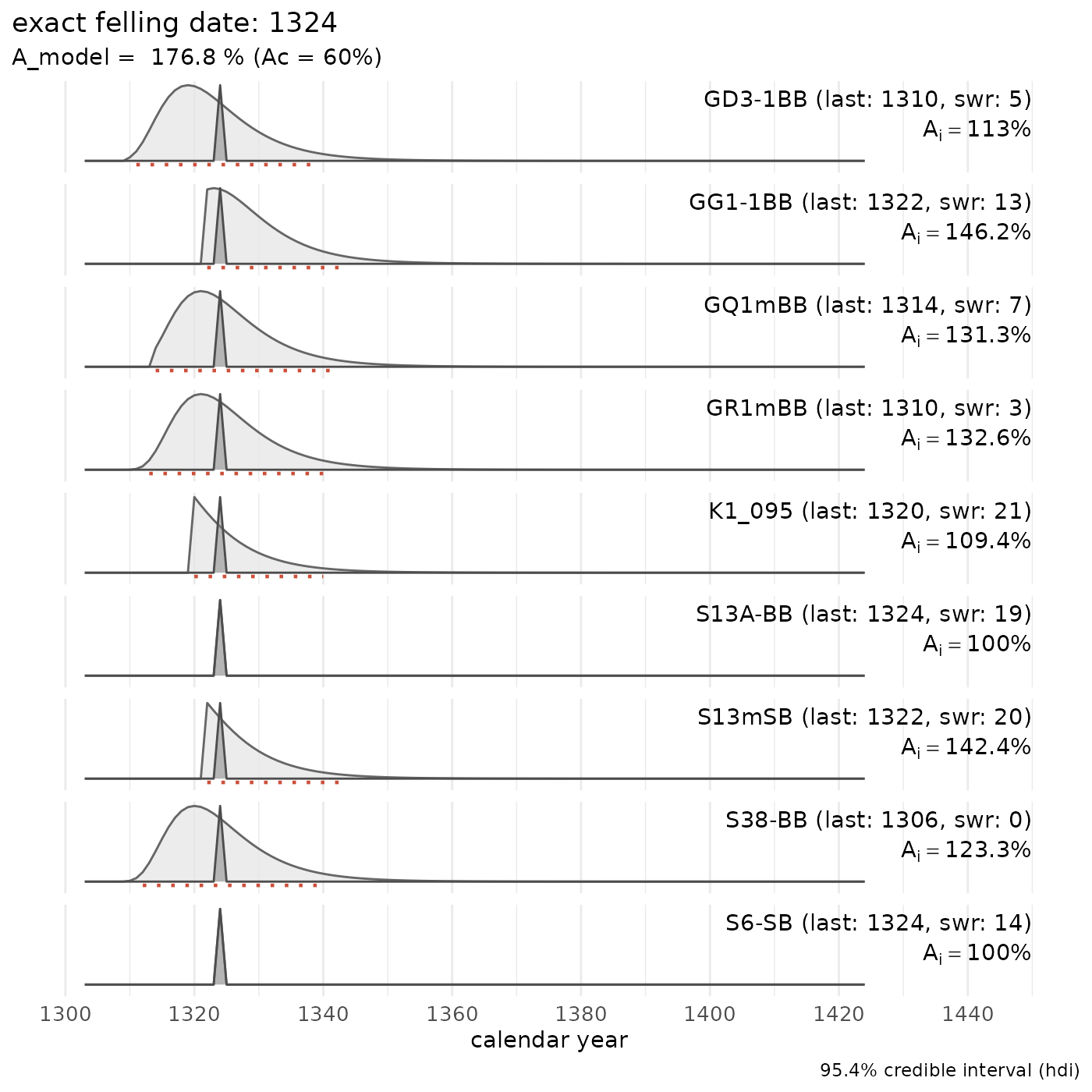
For more details see: Haneca & Daly (2014)
cor_table
The cor_table() function computes common correlation
values between dated tree-ring series (x) and a set of reference
chronologies (y). This function assists in checking the end date of the
series against absolutely dated reference chronologies, but also to
select the most appropriate sapwood model for your data according to the
provenance of the wood (by running it against chronologies that
represent a geographically confined region).
The correlation values computed are:
glk: ‘Gleichläufigkeit’ or ‘percentage of parallel variation’ (Buras & Wilmking 2015; Eckstein & Bauch 1969; Huber 1943; Visser 2020)
glk_p: significance level associated with the glk-value (Jansma 1995)
r_pearson: the Pearson’s correlation coefficient
t_St: Student’s t-value
t_BP: t-values according to the Baillie & Pilcher (1973) algorithm
t_Ho: t-values according to the Hollstein (1980) algorithm
Doel1 <- system.file("extdata", "DOEL1.fh", package = "fellingdater")

Doel1_trs <- read_fh(Doel1, verbose = FALSE)

# crossdating ring-width series from Doel 1 against each other:
cor_results <- cor_table(Doel1_trs, output = "table", min_overlap = 80)
#> Warning in cor_table(Doel1_trs, output = "table", min_overlap = 80): Please use the function `trs_crossdate(x, y, sliding = FALSE)`
#>             instead of `cor_table()`.
#>             For sliding correlations, use `trs_crossdate(x, y, sliding = TRUE)`.
#>             See`?trs_crossdate()` for more information and help
head(cor_results, 20)
#>     series length first last reference ref_first ref_last overlap  glk
#> 29 GD3-1BB     89  1222 1310    GQ1mBB      1150     1314      89 52.8
#> 73 GD3-1BB     89  1222 1310    S13mSB      1164     1322      89 48.9
#> 91 GD3-1BB     89  1222 1310     S6-SB      1221     1324      89 54.5
#> 58 GD3-1BB     89  1222 1310    K1_095      1207     1320      89 51.7
#> 31 GD3-1BB     89  1222 1310    GR1mBB      1220     1310      89 47.2
#> 87 GD3-1BB     89  1222 1310    S38-BB      1193     1306      85 54.2
#> 75 GG1-1BB     83  1240 1322    S13mSB      1164     1322      83 59.8
#> 69 GG1-1BB     83  1240 1322   S13A-BB      1232     1324      83 55.5
#> 59 GG1-1BB     83  1240 1322    K1_095      1207     1320      81 50.6
#> 98 GG1-1BB     83  1240 1322     S6-SB      1221     1324      83 47.0
#> 33  GQ1mBB    165  1150 1314    GR1mBB      1220     1310      91 76.7
#> 76  GQ1mBB    165  1150 1314    S13mSB      1164     1322     151 59.0
#> 60  GQ1mBB    165  1150 1314    K1_095      1207     1320     108 56.1
#> 47  GQ1mBB    165  1150 1314    K1_091      1158     1292     135 60.1
#> 62  GQ1mBB    165  1150 1314   S13A-BB      1232     1324      83 54.9
#> 89  GQ1mBB    165  1150 1314    S38-BB      1193     1306     114 49.6
#> 95  GQ1mBB    165  1150 1314     S6-SB      1221     1324      94 54.3
#> 77  GR1mBB     91  1220 1310    S13mSB      1164     1322      91 65.0
#> 51  GR1mBB     91  1220 1310    K1_095      1207     1320      91 60.0
#> 92  GR1mBB     91  1220 1310     S6-SB      1221     1324      90 55.6
#>           glk_p    r_pearson        t_St  t_BP  t_Ho
#> 29 5.919436e-01 -0.249779208 -2.40605037  2.11  2.74
#> 73 1.169772e+00  0.201284974  1.91669069  1.48  1.97
#> 91 3.910942e-01  0.035883266  0.33491251  2.16  1.92
#> 58 7.477459e-01  0.258187935  2.49273359  0.78  1.71
#> 31 1.408056e+00 -0.370271866 -3.71792327  0.78  1.18
#> 87 4.423117e-01  0.426532081  4.29630804  0.20  0.00
#> 75 7.546208e-02 -0.005084336 -0.04575962  2.28  2.93
#> 69 3.173465e-01  0.217882020  2.00920920  1.06  2.06
#> 59 9.104270e-01  0.597953189  6.63071551  0.09  1.07
#> 98 1.421457e+00 -0.137136419 -1.24599977  0.27  0.78
#> 33 3.624784e-07  0.727924641 10.01554116 12.23 10.41
#> 76 2.697516e-02  0.572471464  8.52261829  5.84  5.40
#> 60 2.067270e-01 -0.282768827 -3.03515368  3.52  3.02
#> 47 1.922538e-02  0.151940473  1.77284639  2.28  2.67
#> 62 3.740983e-01 -0.041724848 -0.37585094  2.19  2.48
#> 89 1.075278e+00 -0.178020527 -1.91457410  2.74  2.34
#> 95 4.042757e-01  0.078494804  0.75522595  1.09  1.16
#> 77 4.212192e-03  0.182334033  1.74946269  4.02  4.24
#> 51 5.640693e-02 -0.248806924 -2.42344980  3.38  3.50
#> 92 2.864524e-01  0.286284295  2.80290094  0.80  0.91