This vignette is a lengthy version of a paper published in The Journal of Open Source Software.
Summary
Tree-ring dating, or dendrochronology, allows the assignment of calendar-year dates to growth rings that can be observed on a cross-section of a stem or a piece of timber. It involves measuring the width of each growth ring and comparing the measured ring-width pattern to absolutely dated reference chronologies. Once a tree-ring series is securely anchored to a calendar year time scale, the end date of the outermost ring can be used to determine or estimate the year of death of the parent tree (i.e., the felling of the tree).
The fellingdater package offers a suite of functions
that can assist dendrochronologists to infer, combine and report felling
date estimates from dated tree-ring series of (pre-)historical timbers,
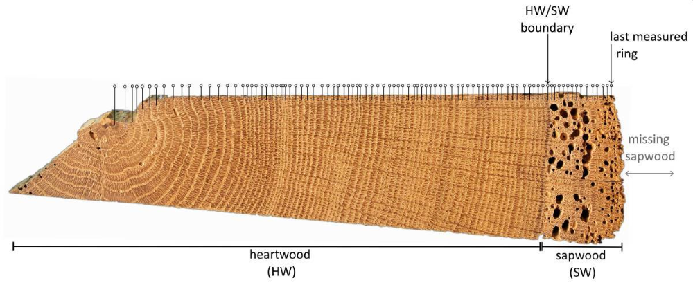
based on the presence of partially preserved sapwood or waney edge (Fig. 1).
Background
Dendrochronology is the most precise chronometric dating technique for (pre-)historical wooden constructions and objects (Baillie 1995). It involves recording the ring-width pattern on a cross-section of an ancient wooden element and matching this pattern to absolutely dated reference chronologies, which allows anchoring the recorded tree-ring pattern to an absolute time scale. From a dated tree-ring pattern it is known in which growing season each growth ring has been laid down by the parent tree. In archaeological, architectural of art-historical studies, the primary objective of a dendrochronological survey is to ascertain an accurate estimate of the felling date (or dying-off) of the parent tree from which the timber originates (Haneca et al. 2009; Domínguez-Delmás 2020; Tegel et al. 2022). This felling date is the closest related and datable event to the creation of the wooden object or construction. These precisely dated events serves as the basis for narratives on various aspects, such as timber selection, craftsmanship, workshop practices, trade, provenance, and historical forest management (Domínguez-Delmás et al. 2023).
The exact felling date can be inferred from the calendar year assigned to the most recently formed tree ring prior to the felling or death of the tree. This requires the presence of the last-formed ring on the object or timber under study, enabling tree-ring dating to achieve (sub-)annual chronological resolution. Unfortunately, this prerequisite is often not fulfilled. The wood of the felled tree may have undergone processing, trimming, or biological deterioration leading to the irreversible loss of wood tissue. When the outermost portion of the timber no longer includes the cambial zone (as illustrated in Fig. 1), the timing of the felling date can only be estimated. The most challenging situation is when neither sapwood, nor the transition between heartwood and sapwood, remains on the object or timber under study (Fig. 1, HW/SW boundary). Sapwood comprises the outermost wood tissues of the xylem in a living tree, representing the physiologically active outer portion of the stem or a branch. It is situated between the cambial zone and the (dead) heartwood, and includes several growth rings. If none of the sapwood is retained, an untraceable amount of wood and growth layers has been removed. In such cases, the last measured and dated ring only provides an earliest possible felling date or terminus post quem.
To refine estimates of felling dates, since the early development of tree-ring dating, datasets have been published with counts of sapwood rings on historical timbers and from living trees, providing a framework for estimating the number of missing rings on tree-ring dated wooden elements with partially preserved sapwood. These sapwood datasets, their transformation into a probabilistic model and the confidence intervals they provide are key elements to obtain a reliable estimate of the felling date of a tree-ring dated piece of timber.
The fellingdater package aims to facilitate this process
by providing functions to infer, combine and report felling date
estimates from dated tree-ring series, based on the presence of
(partially) preserved sapwood or waney edge.
Statement of need
Many descriptive statistics and statistical models have been published to establish accurate estimates of the expected number of sapwood ring (Edvardsson et al. 2022; Bleicher et al. 2020; Rybnicek et al. 2006; Pilcher 1987; Hollstein 1965, 1980; Wazny 1990; Miles 1997; Sohar et al. 2012; Bräthen 1982; Haneca et al. 2009; Hughes et al. 1981; Jevšenak et al. 2019; Hillam et al. 1987; Gjerdrum 2013; Shindo et al. 2024). These models are based on counts of sapwood rings from living and historical timber and often rely on log-transformation of the original data, or use regression models including additional variables such as mean ring width, the cambial age of the tree or a combination of both. These statistical procedures report the expected minimal and maximal number of sapwood rings, usually within 95% a confidence interval, but have also been presented in a wide variety of ways and differ among laboratories and dendrochronologists. A standardized methodology for reporting felling dates is therefore hampered by this variety in statistical approaches. This variety in methodology and reporting comes even more to the surface when tree-ring dates of multiple elements from a single object, construction or building phase are combined into a single felling date for the whole ensemble. The goal of such a mutual interpretation of the individual felling dates is to refine the range of the felling date, but also to check or test whether these dated tree-ring series/wooden elements could indeed represent one single event (i.e. the felling of trees).
A Bayesian method to improve the procedures to model sapwood data,
compute lower and upper limits for the felling date based upon the
selected sapwood model and a given credible interval have been
introduced by Millard (2002). This
procedure was further refined by Miles
(2006), and critically reviewed with real-life examples by Tyers (2008). This workflow has been
incorporated in OxCal, the routine
software for calibration and analysis of radiocarbon dates and related
archaeological and chronological information (Bronk Ramsey 2009: https://c14.arch.ox.ac.uk/oxcalhelp/Sapwood.html).
Tree-ring analyses, on the other hand, relies on a growing set of
R-packages, with the ‘Dendrochronology Program Library in R’
(Bunn 2008, 2010; Bunn, Korpela, et al.
2022), the dplR-package, at its core (see https://opendendro.org/, Bunn, Anchukaitis, et al.
2022). Yet, the Bayesian methodology to establish sapwood
estimates and felling dates was so far not available as a suite of
functions in R (R Core Team 2022).
In order to facilitate and standardize the reporting, interpretation
and combination of felling dates from historical timbers and objects,
the fellingdater R-package was devised. The package allows
to fully document the methodology to establish a felling date – for a
single timber or a group of timbers – making the whole procedure
reproducible and assists in building standardized workflows when applied
to large datasets of historical tree-ring series originating from
geographically distinct regions (e.g. Haneca et
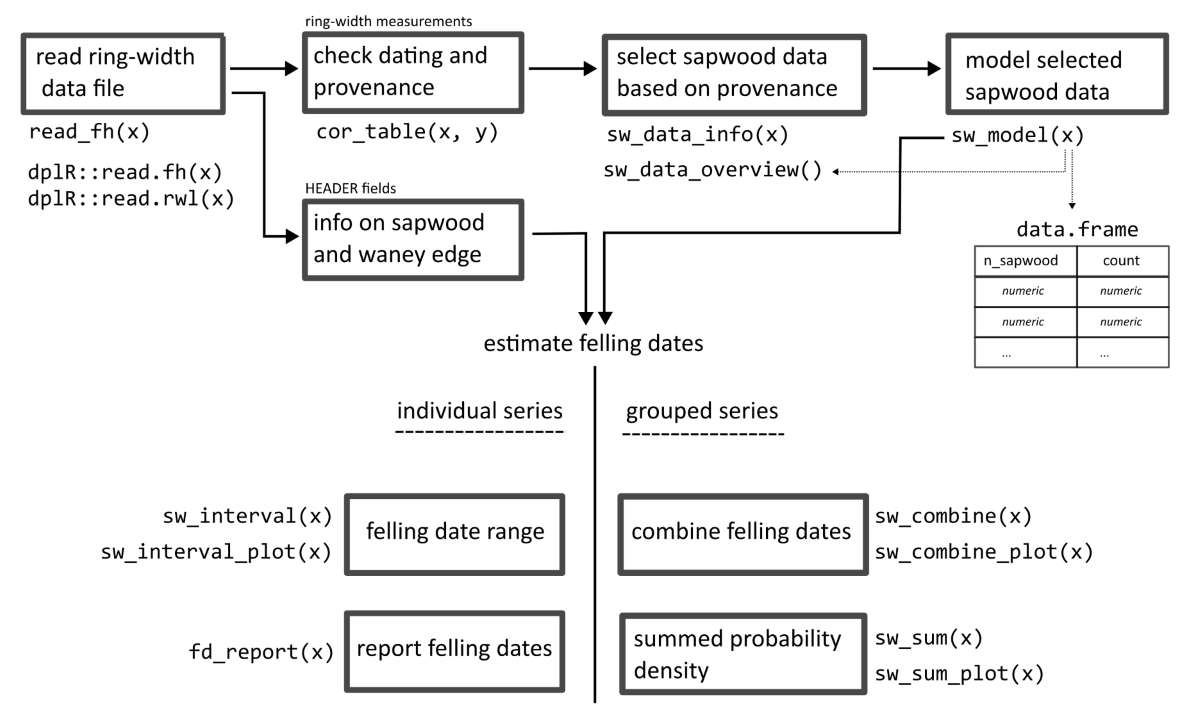
al. 2020). The package is designed to offer several functions
that are related to each step in the (generalized) workflow when
analysing tree-ring series from (pre-)historical objects or
constructions (Fig. 2).
Data within the package
The package comes with published datasets of sapwood counts. The
original data was in most cases retrieved from the original publication
by digitizing scatter plots or frequency histograms (e.g. Haneca and Debonne 2012). This was only
possible for a limited number of publications as many of those datasets
have been published as histograms with wide bins (>1), what does do
not allow to retrieve the underlying data points. An overview of all
currently available sapwood datasets included in the package is
generated by sw_data_overview().
More information on the datasets, such as the bibliographic reference
to the original publication, the wood species and some basic descriptive
statistics (sample size, mean, median, min-max, …) can be retrieved, for
instance, by sw_data_info("Hollstein_1980").
sw_model() fits a density distribution (lognormal,
normal, weibull or gamma) to the original data, and returns the output
iof the modelling process. With sw_model_plot() the model
is visualized as a ggplot-style graph (Wickham
2016) (Fig. 3).
# The function `sw_data_overview()` returns an overview of all available sapwood datasets
# distributed with the package:
sw_data_overview()
#>  [1] "Brathen_1982"     "Hollstein_1980"   "Miles_1997_NM"    "Miles_1997_SC"
#>  [5] "Miles_1997_WBC"   "Pilcher_1987"     "Sohar_2012_ELL_c" "Sohar_2012_ELL_t"
#>  [9] "Sohar_2012_FWE_c" "Sohar_2012_FWE_t" "Wazny_1990"       "vanDaalen_NLBE"
#> [13] "vanDaalen_Norway"

# Use one of the names given by 'sw_data_overview()' as an argument inside
#`sw_data_info()'to obtain information on the dataset (citation, area covered,
# n_observations, and summary_raw_data)

sw_data_info("Pilcher_1987")
#> $data
#> [1] "Pilcher_1987"
#>
#> $citation
#> [1] "Pilcher J.R. 1987. A 700 year dating chronology for northern France.
#> Applications of tree-ring studies. Current research in dendrochronology and
#> related subjects. BAR International Series 333, 127–139."
#>
#> $area
#> [1] "Northern France"
#>
#> $n_observations
#> [1] 116
#>
#> $summary_raw_data
#>    Min. 1st Qu.  Median    Mean 3rd Qu.    Max.
#>   12.00   22.00   26.00   26.72   31.00   49.00

# Pick the dataset most suited for your case-study and fit a (log-)normal, weibul,
# or gamma distribution to the data.

model <- sw_model("Hollstein_1980", plot = FALSE)
sw_model_plot(model)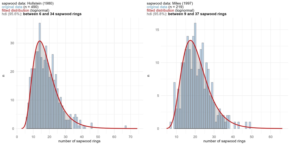
Example of use
The following examples will walk you through the workflow of reading and crossdating ring-width series (Fig. 2), selecting the appropriate sapwood data and modelling options, and finally computing estimates of felling dates and reporting the outcome of this procedure, both for single series as for a group of related tree-ring series.
Installation
The latest version of the package is hosted on GitHub and R-universe, and can be installed locally:
# install.packages("pak")
pak::pak("ropensci/fellingdater")
or
install.packages("fellingdater", repos = "https://ropensci.r-universe.dev")Reading tree-ring files
The function read_fh() is an extension to the
dplR::read.fh() function and allows to read .fh (format
Heidelberg) files of ring widths (in decadal, half-chrono or chrono
format) (Brewer and Murphy 2011), but is
more focused on extracting additional information found in the HEADER
fields of the .fh files. These HEADER fields often harbour essential
information necessary for establishing a well informed estimate of the
felling date, such as the measured number of sapwood rings, the number
of observed but unmeasured rings, the presence of the HW/SW boundary,
the presence of the cambial zone, etc. The read_fh()
function retrieves the information from the HEADER fields and lists the
items as attributes to the ring-width measurements. The
fh_header()function facilitates easy conversoin to a
data.frame.
In the example below, an .fh file with ring-width measurements on
timbers from a medieval ship DOEL1 (Haneca and
Daly 2014) is read with read_fh().
Doel1 <- system.file("extdata", "DOEL1.fh", package = "fellingdater")

# When header = TRUE, the get_header() function is triggered and HEADER fields
# in the .fh file are returned as a data.frame, instead of the ring-width
# measurements.

Doel1_header <- read_fh(Doel1, verbose = FALSE, header = TRUE)
dplyr::glimpse(Doel1_header)

# Columns: 29
# $ series            <chr> "K1_091", "S38-BB", "GD3-1BB", "GR1mBB", "S13mSB", "S13A-BB"
# $ data_type         <chr> "Single", "Single", "Single", "Quadro", "Quadro", "Single"
# $ chrono_members    <chr> NA, NA, NA, "K1_001,K1_004x,GR1-3BB", "S1-3SB,K1_076", NA
# $ species           <chr> "QUSP", "QUSP", "QUSP", "QUSP", "QUSP", "QUSP"
# $ first             <dbl> 1158, 1193, 1222, 1220, 1164, 1232
# $ last              <dbl> 1292, 1306, 1310, 1310, 1322, 1324
# $ length            <dbl> 135, 114, 89, 91, 159, 93
# $ n_sapwood         <dbl> 15, 0, 5, 3, 20, 19
# $ n_sapwood_chr     <chr> NA, NA, NA, NA, NA, NA
# $ unmeasured_rings  <dbl> NA, NA, NA, NA, NA, NA
# $ invalid_rings     <dbl> NA, NA, NA, NA, NA, 1
# $ status            <chr> "Dated", "Dated", "Dated", "Dated", "Dated", "Dated"
# $ waneyedge         <chr> NA, NA, NA, NA, NA, "WKE"
# $ bark              <chr> NA, NA, NA, NA, NA, NA
# $ pith              <chr> "-", "-", "-", "-", "-", "-"
# $ pith_offset       <dbl> NA, NA, NA, NA, NA, NA
# $ pith_offset_delta <dbl> NA, NA, NA, NA, NA, NA
# $ comments          <chr> "keelplank", "framing timber", "hull plank", ...
# $ project           <chr> "Ship timbers DOEL 1", "Ship timbers DOEL 1", ...
# $ location          <chr> "Doel_Deurganckdok", "Doel_Deurganckdok", ...
# $ town              <chr> NA, NA, NA, "Doel", NA, NA
# $ zip               <chr> NA, NA, NA, NA, NA, NA
# $ street            <chr> NA, NA, NA, "Deurganckdok", NA, NA
# $ sampling_date     <chr> NA, NA, NA, NA, NA, NA
# $ measuring_date    <chr> NA, NA, NA, NA, NA, NA
# $ personal_id       <chr> "KH", "KH", "KH", "KH", "KH", NA
# $ client_id         <chr> NA, NA, NA, NA, NA, NA
# $ longitude         <chr> "4.269711", "4.269711", "4.269711", ...
# $ latitude          <chr> "51.298236", "51.298236", "51.298236", ...
Crossdating
The function cor_table() computes commonly used
correlation values between dated tree-ring series and reference
chronologies. This function helps to check the assigned end date of the
series by comparing the measurements against absolutely dated reference
chronologies. This might also provide more information on timber
provenance, as some reference chronologies represent a geographically
confined region. Such information allows to select the most appropriate
sapwood model for your tree-ring data according to the provenance of the
wood.
The correlation values computed are:
glk: ‘Gleichläufigkeit’ or ‘percentage of parallel variation’ (Buras and Wilmking 2015; Eckstein and Bauch 1969; Huber 1943; Visser 2021).
glk_p: significance level associated with the glk-value (Jansma 1995).
r_pearson: the Pearson’s correlation coefficient.
t_St: Student’s t-value based on r_pearson.
t_BP: t-values according to the algorithm proposed by Baillie and Pilcher (1973).
t_Ho: t-values according to the algorithm proposed by Hollstein (1980).
Doel1_trs <- read_fh(Doel1, header = FALSE)
Hollstein_crn <- read_fh("Hollstein80.fh", header = FALSE)

cor_table(x = Doel1_trs,
          y = Hollstein_crn,
          min_overlap = 80, # sets the minimum overlap between series and reference
          output = "table",
          sort_by = "t_BP")
Felling date interval
After selecting the appropriate sapwood model (e.g., one of Fig. 3) one can use the model to estimate the
upper and lower limits of the number of missing sapwood rings. The
function sw_interval() calcualtes the probability density
function (PDF) and highest probability density interval (HDI) of the
felling date range based on the observed number of sapwood rings
(n_sapwood = ...), their chronological dating
(last = ...) and the selected sapwood data
(sw_data = ...) and model (densfun = ...).
In the example below, 10 sapwood rings were observed on a historical
timber, with the last ring dated to 1234 CE, that is supposed to have a
provenance in the Southern Baltic region (covered by the sapwood model
published by Wazny (1990)). The HDI
delineates an interval in which the actual felling date is most likely
situated. It is the shortest interval within a probability distribution
for a given probability mass or credible interval
(cred_mass = ...). The HDI summarizes the distribution by
specifying an interval that spans most of the distribution (in the
example below the credible interval is set to 95%), as such that every
point inside the interval has higher credibility than any point outside
the interval (Fig. 4).
Note that the more sapwood rings that have been measured, the more probability mass is assigned to the tails of the sapwood model.
# 10 sapwood rings observed and the Wazny 1990 sapwood model:

interval <- sw_interval(
     n_sapwood = 10,
     last = 1234,
     hdi = TRUE,
     cred_mass = .95,
     sw_data = "Wazny_1990",
     densfun = "lognormal",
     plot = TRUE)
Reporting individual series
Reporting estimates of the felling date range for multiple individual
series, is conveniently provided by the function
fd_report(). The column felling_date in the
data.frame that is returned, reports the felling date in
verbatim.
df <- data.frame(id = c("trs1", "trs2", "trs3"),
                 swr = c(10, 11, 12),
                 waneyedge = c(FALSE, FALSE, TRUE),
                 end = c(123, 456, 1789)
                 )

fd_report(df,
         series = "id",
         n_sapwood = "swr",
         last = "end",
         sw_data = "Wazny_1990")

#>   series last n_sapwood waneyedge lower upper        felling_date sapwood_model
#> 1    aaa  123        10     FALSE   123   139 between 123 and 139    Wazny_1990
#> 2    bbb  456        11     FALSE   456   471 between 456 and 471    Wazny_1990
#> 3    ccc 1789        12      TRUE    NA  1789             in 1789    Wazny_1990
Combine felling dates
The procedure to combine felling dates of a group of related
tree-ring series with (partially) preserved sapwood, in order to narrow
down the range of a common felling date is provided by the function
sw_combine(). This function returns a list
with:
the probability density function (PDF) for the felling date of the individual series and the PDF of the model that combines these individual series (
$data_raw),the HDI for the combined estimate of the common felling date (
$hdi_model),the Agreement index (
$A_model) of the model, expressing how well the individual series fit into the model ,an overview of the felling date range for the individual series (
$individual_series), and their Agreement index (Ai) to the combined model.
The function sw_combine_plot() allows to visualize the
output (or set plot = TRUE in sw_combine(...)
to call the plot function directly).
The rationale and mathematical background of the Agreement index (Ai)was introduced and developed by Bronk Ramsey (1995, 2017). Both the Ai of the individual series as for the whole model (Amodel) should ideally be around 100%, and not lower than the critical threshold Ac = 60%.
The procedure of testing whether a group of timbers might share a common felling date based on their tree-ring patterns is demonstrated in the next section, with an example dataset consisting of 5 dated tree-ring series of which one has an exact felling date (Fig. 5, left). The proposed felling date (dark grey distribution) equals the felling date of the series with an exact felling date (sw_15), but now it can be assessed that this falls within the felling date ranges for three other individual series (trs_11, trs_12 and trs_14). One other series (trs_13) has no remaining sapwood and therefore only a terminus post quem (earliest possible felling date) can be given (arrow pointing away from last measured ring). The agreement indexes of all individual series and the overall model are high and above the critical threshold of 60%.
sw_example2
#>   series last n_sapwood waneyedge
#> 1 trs_11 1000         5     FALSE
#> 2 trs_12 1005        10     FALSE
#> 3 trs_13 1008        NA     FALSE
#> 4 trs_14 1000         1     FALSE
#> 5 trs_15 1010         3      TRUE

p1 <- sw_combine(sw_example2, plot = TRUE)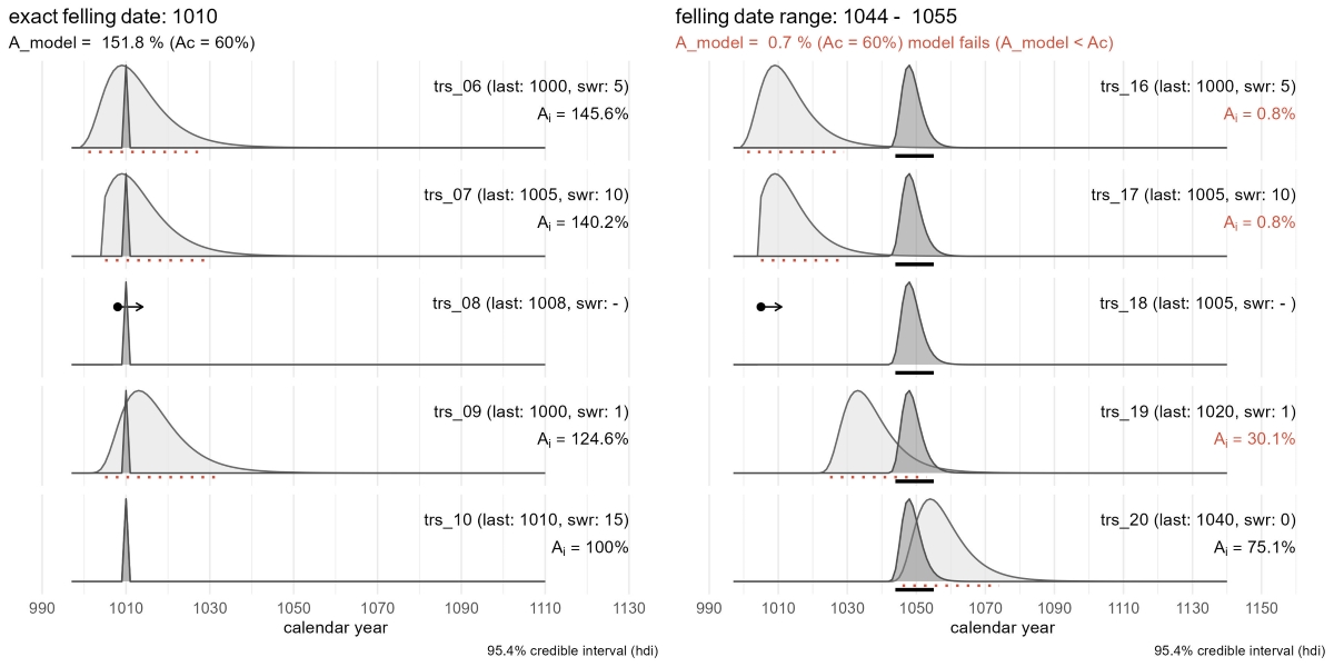
sw_combine(). The sapwood model for the individual series
in light grey, the probability density function of the combined felling
in dark grey tone. The credible interval for the felling date of
individual series is shown as a dashed red line and a black line for the
combined estimate. The dataset in the left graph includes an exact
felling date that matches with the estimates for the other series. The
graph on the right shows a model that fails to group all series around a
common felling date.In the next example, an attempt to compute a common felling date for a group of 5 tree-ring series fails. All but one of the series include partially preserved sapwood, but these tree-ring series do not share a common timing for their estimated felling date (Fig. 5, right). The agreement index of the model is far below 60%, as is the case for most of the individual series. In this particular example, probably two or three separate felling events are present.
sw_example4
#>   series last n_sapwood waneyedge
#> 1 trs_21 1000         5     FALSE
#> 2 trs_22 1005        10     FALSE
#> 3 trs_23 1005        NA     FALSE
#> 4 trs_24 1020         1     FALSE
#> 5 trs_25 1040         0     FALSE

p2 <- sw_combine(sw_example4, plot = TRUE)
Sum felling dates
For large datasets of dated tree-ring series, it is not always
straightforward to assess temporal trends in the frequency of felling
dates. Exact felling dates can be stacked by calender year, but for
series with partially preserved sapwood, their felling date is situated
in an interval. The individual series each have their own probability
density function based on a chosen sapwood model and the number of
observed sapwood rings. To make another reference to radiocarbon dating,
it is common practice in the analysis of large volumes of radiocarbon
dates to compute the summed probability densities (SPD) of the
calibrated radiocarbon dates. Summed probabilities are used to determine
the temporal density of ages (events) in situations where there is no
clear prior information on their distribution (Bronk Ramsey 2017). This procedure is
implemented in OxCal and the R-package rcarbon (Crema and Bevan 2020). The function
sw_sum() makes his procedure available for tree-ring
analyses. The summed probability distribution (SPD) of the individual
probability densities of felling dates of single tree-ring series with
incomplete sapwood allows to visualize fluctuations in the incidence of
potential felling dates over time. The resulting p-values
should however not be interpreted in a probabilistic way but must be
regarded as relative measures that unveil temporal trends in the
dataset. Exact felling dates derived from tree-ring series with waney
edge are not included in the computational process of the SPD as they
would result in anomalous spikes in the SPD, as their associated
probability (p = 1) would be assigned to a single calendar
year, whereas for series with incomplete sapwood the total probability
(p = 1) is dispersed over a wider time range. Therefore exact
felling dates are plotted separately on top of the SPD (Fig. 6).
sum <- sw_sum(sw_example7)

sw_sum_plot(sum, dot_size = 2, dot_shape = 25)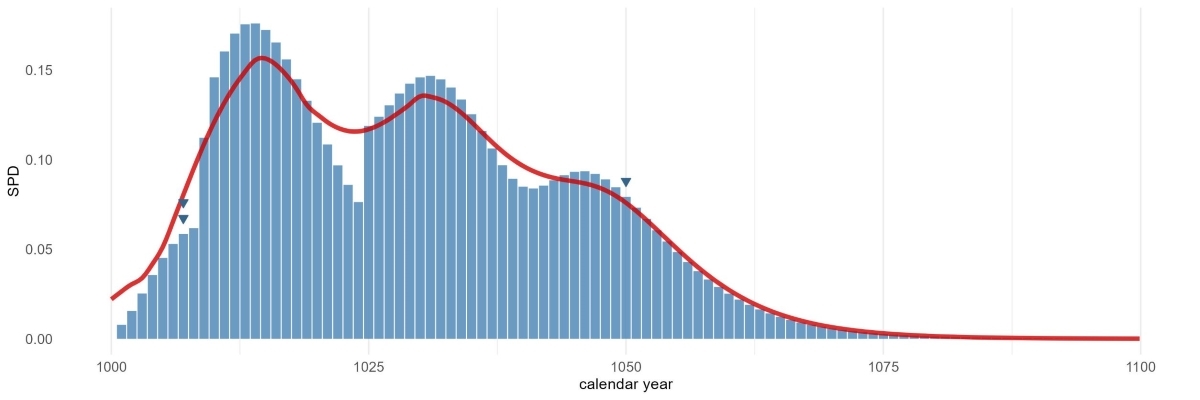
sw_sum(). The blue bars represent the summed probability
density (SPD) of the individual series with partial sapwood. The red
line is a window filter applied to the SPD to highlight the general
trend. Series with exact felling dates (presence of waney edge) are
plotted as triangles above the blue bars of the SPD.Future work
In its current version the package fellingdater is
tailored to the general workflow for analyzing tree-ring datasets from
wooden cultural heritage objects and constructions, made of European oak
(Quercus sp.). The sapwood data included in the current version
reflect this focus on oak. However, all functions can also work with a
custom sapwood dataset provided as a data.frame, with
columns named n_sapwood and count. The latter
reporting the number of occurrences a certain number of sapwood rings
(n_sapwood) was observed on a timber or core sample from
the reference dataset. As such, sapwood data from other regions and
species can also be explored, modeled and used to determine felling
dates by the users of fellingdater.
When new datasets of sapwood counts become available, these can be incorporated in future versions of the package.
Acknowledgements
Koen Van Daele and Ronald Visser fueled me with valuable feedback on earlier versions of the package.
At rOpenSci, dr. Antonio J. Pérez-Luque, dr. Nicholas Tierney and dr. Maëlle Salmon provided an essential and constructive software review, allowing me to significantly improve the quality of the package.