dynamite: An R Package for Dynamic Multivariate Panel Models

dynamite is an R package for Bayesian inference of intensive panel (time series) data comprising multiple measurements per multiple individuals measured in time. The package supports joint modeling of multiple response variables, time-varying and time-invariant effects, a wide range of discrete and continuous distributions, group-specific random effects, latent factors, and customization of prior distributions of the model parameters. Models in the package are defined via a user-friendly formula interface, and estimation of the posterior distribution of the model parameters takes advantage of state-of-the-art Markov chain Monte Carlo methods. The package enables efficient computation of both individual-level and aggregated predictions and offers a comprehensive suite of tools for visualization and model diagnostics. This vignette is a modification of (Tikka and Helske 2024a).

1 Introduction

Panel data is common in various fields such as social sciences. These data consist of multiple individuals followed over several time points, and there are often many observations per individual at each time, for example, family status and income of each individual at each time point of interest. Such data can be analyzed in various ways, depending on the research questions and the characteristics of the data such as the number of individuals and time points, and the assumed distribution of the response variables. In social sciences, popular, somewhat overlapping modeling approaches include dynamic panel models, fixed effect models, dynamic structural equation models (Asparouhov, Hamaker, and Muthén 2018), cross-lagged panel models (CLPM), and their various extensions such as CLPM with fixed or random effects (Arellano and Bond 1991; Allison 2009; Bollen and Brand 2010; Allison, Williams, and Moral-Benito 2017; Hamaker, Kuiper, and Grasman 2015; Mulder and Hamaker 2021) and general cross-lagged panel model (Zyphur et al. 2020).

There are several R (R Core Team 2023) packages available from the Comprehensive R Archive Network (CRAN) focusing on the analysis of panel data. The plm package (Croissant and Millo 2008) provides various estimation methods and tests for linear panel data models, while the fixest package (Bergé 2018) supports multiple fixed effects and different distributions of response variables. The panelr package (Long 2020) contains tools for panel data manipulation and estimation methods for so-called “within-between” models that combine fixed effect and random effect models. This is done by using lme4, geepack, and brms packages as a backend (Bates et al. 2015; Halekoh, Højsgaard, and Yan 2006; Bürkner 2018). The lavaan package (Rosseel 2012) provides methods for general structural equation modeling (SEM) and thus can be used to estimate various panel data models such as CLPMs with fixed or random intercepts. Similarly, it is also possible to use general multilevel modeling packages such as lme4 and brms directly for panel data modeling. Of these, only lavaan and brms support joint modeling of multiple interdependent response variables, which is typically necessary for multi-step predictions and long-term causal effect estimation (Helske and Tikka 2024).

In traditional panel data models such as the ones supported by the aforementioned packages, the number of time points considered is often assumed to be relatively small, say less than 10, while the number of individuals can be hundreds or thousands (Wooldridge 2010). This is especially true for commonly used “wide format” SEM approaches that are unable to consider a large number of time points (Asparouhov, Hamaker, and Muthén 2018). Perhaps due to the small number of time points, the effects of covariates are typically assumed to be time-invariant, although some extensions to time-varying effects have emerged (e.g., Sun, Carroll, and Li 2009; Asparouhov, Hamaker, and Muthén 2018; Hayakawa and Hou 2019). On the other hand, when the number of time points is moderate or large, say hundreds or thousands (sometimes referred to as intensive longitudinal data), it can be reasonable to assume that the dynamics of the system change over time, for example in the form of time-varying effects.

Modeling time-varying effects in (generalized) linear models can be based on state-space models (SSMs, Harvey and Phillips 1982; Durbin and Koopman 2012; Helske 2022), for which there are various R implementations such as walker (Helske 2022), shrinkTVP (Knaus et al. 2021), and CausalImpact (Brodersen et al. 2014). However, these implementations are restricted to a non-panel setting of a single individual and a single response variable. Other approaches include methods based on varying coefficients models (Hastie and Tibshirani 1993; Eubank et al. 2004), implemented in tvReg and tvem packages (Casas and Fernández-Casal 2022; Dziak et al. 2021). While tvem supports multiple individuals, it does not support multiple response variables per individual. The tvReg package supports only univariate single-individual responses. Also based on SSMs and differential equations, the dynr package (Ou, Hunter, and Chow 2019) provides methods for modeling multivariate dynamic regime-switching models with linear or non-linear latent dynamics and linear-Gaussian observations. Because both multilevel models and SEMs can be defined as SSMs (see e.g., Sallas and Harville 1981; Helske 2017; Chow et al. 2010), other packages supporting general SSMs could be suitable for panel data analysis in principle as well, such as KFAS (Helske 2017), bssm (Helske and Vihola 2021), and pomp (King, Nguyen, and Ionides 2016). However, SSMs are often computationally demanding especially for non-Gaussian observations where the marginal likelihood is analytically intractable, and a large number of individuals can be problematic, particularly in the presence of additional group-level random effects which complicates the construction of the corresponding state space model (Helske 2017).

The dynamite package (Tikka and Helske 2024b) provides an alternative approach to panel data inference which avoids some of the limitations and drawbacks of the aforementioned methods. First, the dynamic multivariate panel data models (DMPMs), introduced by Helske and Tikka (2024) and implemented in the dynamite package support estimation of effects that vary smoothly over time according to Bayesian P-splines (Lang and Brezger 2004), with penalization based on random walk priors. This allows modeling for example the effects of interventions that increase or decrease over time. Second, dynamite supports a wide variety of distributions for the response variables such as Gaussian, Poisson, binomial, and categorical distributions. Third, with dynamite, we can model an arbitrary number of simultaneous measurements per individual. Finally, the estimation is fully Bayesian using Markov chain Monte Carlo (MCMC) simulation via Stan (Stan Development Team 2024b) leading to transparent and interpretable quantification of parameter and predictive uncertainty. A comprehensive comparison between DMPMs and other panel data modeling approaches can be found in (Helske and Tikka 2024).

One of the most defining features of dynamite is its high-performance prediction functionality, which is fully automated, supports multi-step predictions over the entire observed time interval, and can operate at the individual level or group level. This is in stark contrast to packages such as brms where, in the presence of lagged response variables as covariates, obtaining such predictions necessitates the computation of manual stepwise predictions and can pose a challenge even for an experienced user. Furthermore, by jointly modeling all endogenous variables simultaneously, dynamite allows us to consider the long-term effects of interventions that take into account the interdependence of the variables in the model.

The paper is organized as follows. In Section 2 we introduce the dynamic multivariate panel model which is the class of models considered in the dynamite package and describe the assumptions made in the package with respect to these models. Section 3 introduces the software package and its core features along with two illustrative examples using a real dataset and a synthetic dataset. Sections 4 and 5 provide a more comprehensive and technical overview of how to define and estimate models using the package. The use of the model fit objects for prediction is discussed in Section 6. Finally, Section 7 summarizes our contributions and provides some concluding remarks.

2 The dynamic multivariate panel model

Consider an individual \(i\) at time \(t\) with observations \(y_{t,i} = (y_{1,t,i},\ldots, y_{C,t,i})\), \(t=1,\ldots,T\), \(i = 1,\ldots,N\). In other words, at each time point \(t\) we have \(C\) observations from \(N\) individuals, where \(C\) is the number of different response variables that have been measured, which we call channels. The response variables can be univariate or multivariate. We assume that each element of \(y_{t,i}\) can depend on the past observations \(y_{t-\ell,i}\), \(\ell=1,\ldots\) (where the set of past values can be different for each channel) and also on additional exogenous covariates \(x_{t,i}\). In addition, each response variable \(y_{c,t,i}\) can depend on other observations at the same time point \(t\), i.e., the elements of \(y_{t,i}\), with the following restriction. We assume that the channels can be ordered so that the distribution of \(y_{t,i}\) factorizes according to an ordering \(\pi\) of the responses. We denote the observations at the same time point before observation \(y_{c,t,i}\) in this ordering by \(y_{\pi(c),t,i}\). Thus, the conditional distribution of channel \(c\) is completely defined by the observations at the same time point before the channel in the ordering \(\pi\), past observations, exogenous covariates, and the model parameters for all \(c = 1,\ldots,C\). For simplicity of the presentation, we now assume that all channels are univariate and that the observations of each channel only depend on the previous time points, i.e., \(\ell = 1\) for all channels. The set of all model parameters is denoted by \(\theta\). We treat the first \(L\) timepoints as fixed data, where \(L\) is the highest order of lag dependence in the model. Now, assuming that the elements of \(y_{t,i}\) are conditionally independent given \(y_{t-1,i}\), \(x_{t,i}\), and \(\theta\) we have \[\begin{equation} y_{t,i} \sim p_t(y_{t,i} | y_{1:t-1,i},x_{t,i},\theta) = \prod_{c = 1}^C p_{c,t}(y_{c,t,i} | y_{\pi(c),t,i}, y_{1:t-1,i}, x_{t,i}, \theta), \tag{1} \end{equation}\] where \(y_{1:t-1,i}\) denotes the past values of the response variables across all channels \((y_{1,i},\ldots,y_{t-1,i})\). Importantly, the parameters of the conditional distributions \(p_{c,t}\) can be time-dependent, enabling us to consider the evolution of the dynamics of our system over time.

Given a suitable link function depending on our distributional assumptions, we define a linear predictor \(\eta_{c,t,i}\) for the conditional distribution \(p^c_t\) of each channel \(c\) with the following general form: \[\begin{equation} \eta_{c,t,i} = \alpha_{c,t} + u^\top_{c,t,i} \beta_c + w^\top_{c,t,i} \delta_{c,t} + z^\top_{c,t,i} \nu_{c,i} + \lambda^\top_{c,i} \psi_{c,t}, \tag{2} \end{equation}\] where \(\alpha_{c,t}\) is the (possibly time-varying) common intercept term, \(u^\top_{c,t,i}\) defines the covariates corresponding to the vector of time-invariant coefficients \(\beta_c\), and similarly \(w^\top_{c,t,i}\) defines the covariates for the time-varying coefficients \(\delta_{c,t}\). The term \(z^\top_{c,t,i} \nu_{c,i}\) corresponds to individual-specific random effects, where \(\nu_{1,i},\ldots, \nu_{C,i}\) are assumed to follow a zero-mean Gaussian distribution, either with a diagonal or a full covariance matrix. Note that the covariates in \(u^\top_{c,t,i}\), \(w^\top_{c,t,i}\), and \(z^\top_{c,t,i}\) may contain values of other response variables at the same time point that appear before channel \(c\) in the ordering \(\pi\), past observations of the response channels (or transformations of them), or exogenous covariates. Covariates in \(z^\top_{c,t,i}\) can overlap those in \(u^\top_{c,t,i}\) and \(w^\top_{c,t,i}\) resulting in an interpretation for \(\nu_{c,i}\) that corresponds to individual-specific deviations from the population-level effects \(\beta_c\) and \(\delta_{c,t}\), respectively. In contrast, the covariates in \(u^\top_{c,t,i}\) and \(w^\top_{c,t,i}\) should in general not overlap to ensure the identifiability of their respective model parameters. The final term \(\lambda^\top_{c,i} \psi_{c,t}\) is a product of latent individual loadings \(\lambda_{c,i}\) and a univariate latent dynamic factor \(\psi_{c,t}\). The latent factors can be correlated across channels.

For the time-varying coefficients \(\delta_{c,t}\) (and similarly for time-varying \(\alpha_{c,t}\) and the latent factor \(\psi_{c,t}\)), we use Bayesian P-splines such that \[ \delta_{c,t,k} = b^\top_t \omega_{c,k}, \quad k=1,\ldots,K, \] where \(K\) is the number of covariates, \(b_t\) is a vector of B-spline basis function values at time \(t\), and \(\omega_{c,k}\) is a vector of corresponding spline coefficients. We assume a B-spline basis of equally spaced knots on the time interval from \(L+1\) to \(T\) with \(D\) degrees of freedom. In general, the number of B-splines \(D\) used for constructing the splines for the study period \(1,\ldots,T\) can be chosen freely, but the actual value is not too important (as long as \(D\) is larger than the degree of the spline, e.g., three for cubic splines, Wood 2020). Therefore, we use the same \(D\) basis functions for all time-varying effects. To mitigate overfitting due to too large a value of \(D\), we define a random walk prior (Lang and Brezger 2004) for \(\omega_{c,k}\) as \[ \omega_{c,k,1} \sim p(\omega_{c,k,1}), \quad \omega_{c,k,d} \sim N(\omega_{c,k,d-1}, \tau^2_{c,k}), \quad d=2, \ldots, D, \] with a user-defined prior \(p(\omega_{c,k,1})\) on the first coefficient, which due to the structure of \(b_1\) corresponds to a prior on \(\delta_{c,k,1}\). Here, the parameter \(\tau_{c,k}\) controls the smoothness of the spline curves. While the different time-varying coefficients are modeled as independent a priori, the latent factors \(\psi_{c,t}\) can be modeled as correlated via correlated spline coefficients \(\omega_{c,k}\). See Appendix A for the details of the parametrization of the latent factor term.

For categorical, multivariate, and other distributions with multiple dimensions or components, we can extend the definition of the linear predictor in Equation (2) to account for each dimension by simply replacing the index \(c\) with indices \(c,s\) where \(s\) denotes the index of the dimension, \(s = 1,\ldots,S(c)\), and \(S(c)\) is the number of dimensions of channel \(c\). This extension also applies to the spline coefficients.

3 The dynamite package

The dynamite package provides an easy-to-use interface for fitting DMPMs in R. As the package is part of rOpenSci (https://ropensci.org), it complies with its rigorous software standards and the development version of dynamite can be installed from the R-universe system (https://ropensci.org/r-universe/). The stable version of the package is available from CRAN at (https://cran.r-project.org/package=dynamite). The software is published under the GNU general public license (GPL \(\geq\) 3) and can be obtained in R by running the following commands:

install.packages("dynamite")
library("dynamite")

The package takes advantage of several other well-established R packages. Estimation of the models is carried out by Stan for which both rstan and cmdstanr interfaces are available (Stan Development Team 2024a; Gabry and Češnovar 2023). More specifically, the MCMC simulation uses the No-U-Turn sampler (NUTS, Hoffman and Gelman 2014) which is an extension of Hamiltonian Monte Carlo (HMC, Neal 2011). The data.table package (Barrett et al. 2024) is used for efficient computation and memory management of predictions and internal data manipulations. For posterior inference and visualization, ggplot2 and posterior packages are leveraged (Wickham 2016; Bürkner et al. 2023). Leave-one-out (LOO) and leave-future-out (LFO) cross-validation methods are implemented with the help of the loo package (Vehtari et al. 2022). All of the aforementioned dependencies are available on CRAN except for cmdstanr whose installation is optional and needed only if the user wishes to use the CmdStan backend for Stan. Although not required for dynamite, we also install the dplyr, pder, and pryr packages (Wickham et al. 2023; Croissant and Millo 2022; Wickham 2023), as we will use them in the subsequent sections.

install.packages(c("dplyr", "pder", "pryr"))

Several example datasets and corresponding model fit objects are included in dynamite which are used throughout this paper for illustrative purposes. The script files to generate these datasets and the model fit objects can be found in the package GitHub repository (https://https://github.com/ropensci/dynamite/) under the data-raw directory. Table 1 provides an overview of the available functions and methods of the package. Before presenting the technical details, we demonstrate the key features of the package and the general workflow by performing an illustrative analysis on a real dataset and a synthetic dataset.

Table 1: The functionality of dynamite. Asterisks denote "dynamitefit" methods that are also available for "dynamiteformula" objects.

Function	Output	Description
dynamite()	"dynamitefit"	Estimate a dynamic multivariate panel model
dynamice()	"dynamitefit"	Estimate a DMPM with multiple imputation
dynamiteformula()	"dynamiteformula"	Define a response channel
+.dynamiteformula()	"dynamiteformula"	Add definitions to a model formula
obs()	"dynamiteformula"	Define a response channel (alias)
aux()	"dynamiteformula"	Define a deterministic channel
splines()	"splines"	Define P-splines for time-varying coefficients
random_spec()	"random_spec"	Define additional properties of random effects
lags()	"lags"	Define lagged covariates for all channels
lfactor()	"lfactor"	Define latent factors
as.data.frame()	"data.frame"	Extract posterior samples or summaries
as.data.table()	"data.table"	Extract posterior samples or summaries
as_draws()	"draws_df"	Extract posterior samples or summaries
as_draws_df()	"draws_df"	Extract posterior samples or summaries
coef()	"tbl_df"	Extract posterior samples or summaries
confint()	"matrix"	Extract credible intervals
fitted()	"data.table"	Compute fitted values
formula()	"language"	Extract the model formula
get_code()	"data.frame"	Extract the Stan model code*
get_data()	"list"	Extract the data used to fit the model*
get_parameter_dims()	"list"	Extract parameter dimensions*
get_parameter_names()	"character"	Extract parameter names
get_parameter_types()	"character"	Extract parameter types
get_priors()	"data.frame"	Extract the prior distribution definitions*
hmc_diagnostics()	"dynamitefit"	Compute HMC diagnostics
lfo()	"lfo"	Compute LFO cross-validation for the model
loo()	"loo"	Compute LOO cross-validation for the model
mcmc_diagnostics()	"dynamitefit"	Compute MCMC diagnostics
ndraws()	"integer"	Extract the number of posterior draws
nobs()	"integer"	Extract the number of observations
plot()	"ggplot"	Visualize posterior distributions
predict()	"data.frame"	Compute predictions
print()	"dynamitefit"	Print information on the model fit*
summary()	"data.frame"	Print a summary of the model fit
update()	"dynamitefit"	Update the model fit

3.1 Bayesian inference of seat belt usage and traffic fatalities

As the first illustration, we consider the effect of seat belt laws on traffic fatalities using data from the pder package, originally analyzed by Cohen and Einav (2003). The data consists of the number of traffic fatalities and other related variables in the United States from all 51 states for every year from 1983 to 1997. During this time, many states passed laws regarding mandatory seat belt use. We distinguish two types of laws: secondary enforcement law and primary enforcement law. Secondary enforcement means that the police can fine violators only when they are stopped for other offenses, whereas in primary enforcement the police can also stop and fine based on the seat belt use violation itself. This dataset is named SeatBelt and it can be loaded into the current R session by running:

data("SeatBelt", package = "pder")

To begin, we rename some variables and compute additional transformations to make the subsequent analyses straightforward.

library("dplyr")
seatbelt <- SeatBelt |>
  mutate(
    miles = (vmturban + vmtrural) / 10000,
    log_miles = log(miles),
    fatalities = farsocc,
    income10000 = percapin / 10000,
    law = factor(
      case_when(
        dp == 1 ~ "primary",
        dsp == 1 ~ "primary",
        ds == 1 & dsp == 0 ~ "secondary",
        TRUE ~ "no_law"
      ),
      levels = c("no_law", "secondary", "primary")
    )
  )

We are interested in the effect of the seat belt law on traffic fatalities in terms of car occupants via the changes in seat belt usage. For this purpose, we build a joint model for seat belt usage and fatalities. We model the rate of seat belt usage with a beta distribution (with a logit link) and assume that the usage depends on the level of the seat belt law, state-level effects (modeled as random intercepts), and overall time-varying trend (modeled as a spline), which captures potential changes in the general tendency to use a seat belt in the US. We model the number of fatalities with a negative binomial distribution (with a log link) using the total miles traveled as an offset. In addition to the seat belt usage and state-level random intercepts, we also use several other variables related to traffic density, speed limit, alcohol usage, and income (see ?pder::SeatBelt for details) as controls. First, we construct the model formula that defines the distributions of the response channels, the covariates of each channel, and the splines used for the time-varying effects:

seatbelt_formula <-
  obs(usage ~ -1 + law + random(~1) + varying(~1), family = "beta") +
  obs(
    fatalities ~ usage + densurb + densrur +
      bac08 + mlda21 + lim65 + lim70p + income10000 + unemp + fueltax +
      random(~1) + offset(log_miles), 
    family = "negbin"
  ) +
  splines(df = 10)

Next, we fit the model

fit <- dynamite(
  dformula = seatbelt_formula,
  data = seatbelt, time = "year", group = "state",
  chains = 4, refresh = 0
)

We can extract the estimated coefficients with the summary() method which shows clear positive effects for both secondary enforcement and primary enforcement laws:

#> # A tibble: 2 × 5
#>   parameter                mean     sd    q5   q95
#>   <chr>                   <dbl>  <dbl> <dbl> <dbl>
#> 1 beta_usage_lawsecondary 0.495 0.0473 0.416 0.572
#> 2 beta_usage_lawprimary   1.05  0.0864 0.907 1.19

While these coefficients can be interpreted as changes in log-odds as usual, we also estimate the marginal means using the fitted() method which returns the posterior samples of the expected values of the responses at each time point given the covariates. For this purpose, we create a new data frame for each level of the law factor and assign every state to uphold this particular law. We then call fitted() using these data, compute the averages of over the states and finally over the posterior samples:

seatbelt_new <- seatbelt
seatbelt_new$law[] <- "no_law"
pnl <- fitted(fit, newdata = seatbelt_new)
seatbelt_new$law[] <- "secondary"
psl <- fitted(fit, newdata = seatbelt_new)
seatbelt_new$law[] <- "primary"
ppl <- fitted(fit, newdata = seatbelt_new)
bind_rows(no_law = pnl, secondary = psl, primary = ppl, .id = "law") |>
  mutate(
    law = factor(law, levels = c("no_law", "secondary", "primary"))
  ) |>
  group_by(law, .draw) |>
  summarize(mm = mean(usage_fitted)) |>
  group_by(law) |>
  summarize(
    mean = mean(mm),
    q5 = quantile(mm, 0.05),
    q95 = quantile(mm, 0.95)
  )
#> # A tibble: 3 × 4
#>   law        mean    q5   q95
#>   <fct>     <dbl> <dbl> <dbl>
#> 1 no_law    0.359 0.346 0.373
#> 2 secondary 0.468 0.458 0.477
#> 3 primary   0.591 0.566 0.616

These estimates are in line with the results of Cohen and Einav (2003) who report the law effects on seat belt usage as increases of 11 and 22 percentage points for secondary enforcement and primary enforcement laws, respectively.

For the effect of seat belt laws on the number of traffic fatalities, we compare the number of fatalities with 68% seat belt usage against 90% usage. These values, coinciding with the national average in 1996 and the target of 2005, were also used by who reported an increase in annual lives saved as 1500–3000. We do this by comparing the differences in total fatalities across states for each year, and by averaging over the years, again with the help of the fitted() method;

seatbelt_new <- seatbelt
seatbelt_new$usage[] <- 0.68
p68 <- fitted(fit, newdata = seatbelt_new)
seatbelt_new$usage[] <- 0.90
p90 <- fitted(fit, newdata = seatbelt_new)
bind_rows(low = p68, high = p90, .id = "usage") |>
  group_by(year, .draw) |>
  summarize(
    s = sum(
      fatalities_fitted[usage == "low"] -
        fatalities_fitted[usage == "high"]
    )
  ) |>
  group_by(.draw) |>
  summarize(m = mean(s)) |>
  summarize(
    mean = mean(m),
    q5 = quantile(m, 0.05),
    q95 = quantile(m, 0.95)
  )
#> # A tibble: 1 × 3
#>    mean    q5   q95
#>   <dbl> <dbl> <dbl>
#> 1 1553.  787. 2311.

In this example, the model did not contain any lagged responses as covariates, so it was enough to compute predictions for each time point essentially independently using the fitted() method. However, when the responses depend on the past values of themselves or of other channels, as is the case for example in cross-lagged panel models, estimating long-term causal effects such as \(E(y_{t+k} | do(y_t)), k = 1,\ldots\), where \(do(y_t)\) denotes an intervention on \(y_t\) (Pearl 2009), is more complicated. We illustrate this in our next example.

3.2 Causal effects in a multichannel model

We consider the following simulated multichannel data available in the dynamite package and the estimation of causal effects.

head(multichannel_example)
#>   id time          g  p b
#> 1  1    1 -0.6264538  5 1
#> 2  1    2 -0.2660091 12 0
#> 3  1    3  0.4634939  9 1
#> 4  1    4  1.0451444 15 1
#> 5  1    5  1.7131026 10 1
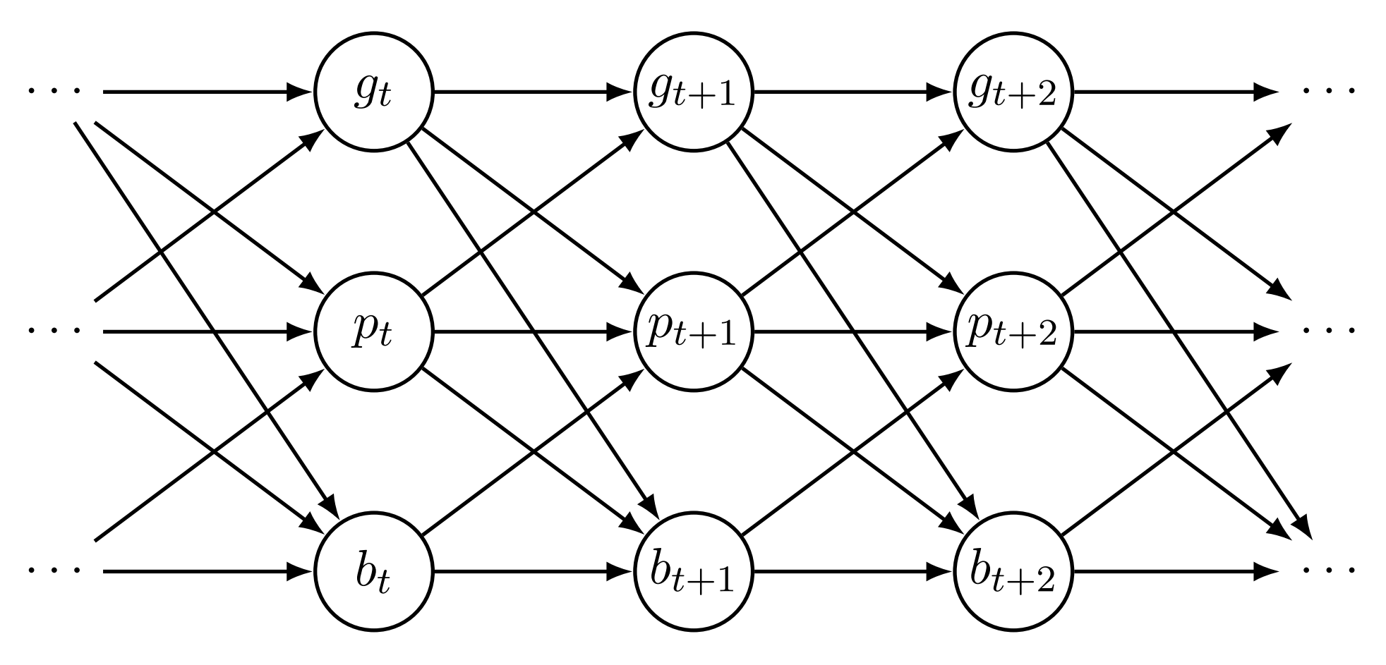
#> 6  1    6  2.1382398  8 1

The data contains 50 unique groups (variable id), over 20 time points (time), a continuous variable \(g_t\) (g), a variable with non-negative integer values \(p_t\) (p), and a binary variable \(b_t\) (b). We define the following model (which actually matches the data-generating process used to generate the data):

multi_formula <- obs(g ~ lag(g) + lag(logp), family = "gaussian") +
  obs(p ~ lag(g) + lag(logp) + lag(b), family = "poisson") +
  obs(b ~ lag(b) * lag(logp) + lag(b) * lag(g), family = "bernoulli") +
  aux(numeric(logp) ~ log(p + 1) | init(0))

Here, the aux() function creates a deterministic transformation of \(p_t\) defined as \(\log(p_t + 1)\) which can subsequently be used in other channels as a covariate and correctly computes the transformation for predictions. Because the model also contains a lagged value of logp, we define the initial value of logp to be 0 at the first time point via the past() declaration. Without the initial value, we would receive a warning message when fitting the model, but in this case we could safely ignore the warning because the model contains lags of b and g as well meaning that the first time point in the model is treated as fixed and does not enter the model fitting process. This makes the past() declaration redundant in this instance, but it is good practice to always define the initial values of deterministic channels when the model contains their lagged values to avoid accidental NA values when the channel is evaluated. A directed acyclic graph (DAG) that depicts the causal relationships of the variables in the model is shown in Figure 1. We fit the model using the dynamite() function.

A directed acyclic graph for the multichannel model with arrows corresponding to the assumed direct causal effects. A cross-section at times \(t\), \(t+1\), and \(t+2\) is shown. The vertices and edges corresponding to the deterministic tranformation \(\log(p_t)\) are omitted for clarity.

multichannel_fit <- dynamite(
  dformula = multi_formula,
  data = multichannel_example, time = "time", group = "id",
  chains = 4, refresh = 0
)

We can obtain posterior samples or summary statistics of the model using the as.data.frame(), coef(), and summary() methods, but here we opt for visualizing the results as depicted in Figure 2 by using the plot() method:

library("ggplot2")
theme_set(theme_bw())
plot(multichannel_fit, types = "beta") +
  labs(title = "")

Figure 2: Posterior means and 90% posterior intervals of the time-invariant coefficients for the multichannel model.

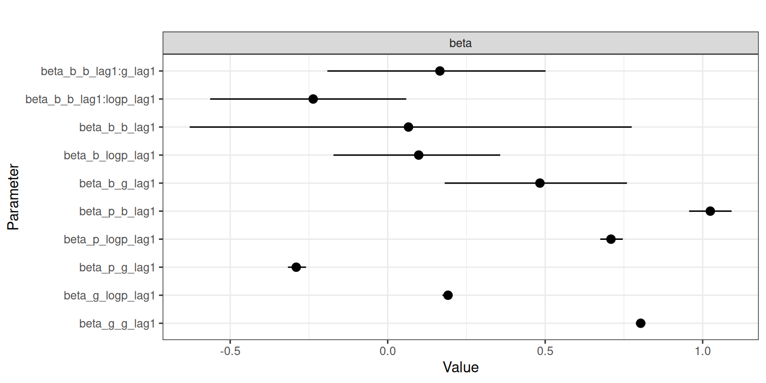
Note the naming of the model parameters; for example, beta_b_g_lag1 corresponds to a time-invariant coefficient beta for channel b of the lagged covariate g.

Assume now that we are interested in the causal effect of \(b_5\) on \(g_t\) at times \(t = 6, \ldots, 20\). There is no direct effect from \(b_5\) to \(g_6\), but because \(g_t\) affects \(b_{t+1}\) (and \(p_{t+1}\)), which in turn affects all variables at \(t+2\), we should see an indirect effect of \(b_5\) to \(g_t\) from time \(t = 7\) onward. For this task, we first create a new dataset where the values of our response variables after time \(t = 5\) are assigned to be missing.

multichannel_newdata <- multichannel_example |>
  mutate(across(g:b, ~ ifelse(time > 5, NA, .x)))

We then obtain predictions for time points \(t = 6,\ldots,20\) when \(b_t\) is assigned to be 0 or 1 for every individual at time \(t = 5\), corresponding to the interventions \(do(b_5 = 0)\) and \(do(b_5 = 1)\).

new0 <- multichannel_newdata |>
  mutate(b = ifelse(time == 5, 0, b))
pred0 <- predict(multichannel_fit, newdata = new0, type = "mean")
new1 <- multichannel_newdata |>
  mutate(b = ifelse(time == 5, 1, b))
pred1 <- predict(multichannel_fit, newdata = new1, type = "mean")

By default, the output from predict() is a single data frame containing the original new data and the samples from the posterior predictive distribution of new observations. By defining type = "mean", we specify that we are interested in the posterior distribution of the expected values instead. In this case, the predicted values in the output are in the columns g_mean, p_mean, and b_mean where the NA values of the newdata argument are replaced with the posterior predictive samples from the model (the output also contains an additional column corresponding to the auxiliary channel logp and posterior draw index variable .draw).

head(pred0, n = 10) |>
  round(3)
#>    id time .draw g_mean p_mean b_mean  logp      g  p  b
#> 1   1    1     1     NA     NA     NA 1.792 -0.626  5  1
#> 2   1    2     1     NA     NA     NA 2.565 -0.266 12  0
#> 3   1    3     1     NA     NA     NA 2.303  0.463  9  1
#> 4   1    4     1     NA     NA     NA 2.773  1.045 15  1
#> 5   1    5     1     NA     NA     NA 2.398  1.713 10  0
#> 6   1    6     1  1.853  3.592  0.698 1.099     NA NA NA
#> 7   1    7     1  1.720  3.736  0.726 1.099     NA NA NA
#> 8   1    8     1  1.666  1.409  0.729 0.693     NA NA NA
#> 9   1    9     1  1.225  1.200  0.706 1.099     NA NA NA
#> 10  1   10     1  1.416  4.148  0.704 1.792     NA NA NA

We can now compute summary statistics over the individuals and then over the posterior samples to obtain the posterior distribution of the expected causal effects \(E(g_t | do(b_5))\) as

sumr <- list(b0 = pred0, b1 = pred1) |>
  bind_rows(.id = "case") |>
  group_by(case, .draw, time) |>
  summarize(mean_t = mean(g_mean)) |>
  group_by(case, time) |>
  summarize(
    mean = mean(mean_t),
    q5 = quantile(mean_t, 0.05, na.rm = TRUE),
    q95 = quantile(mean_t, 0.95, na.rm = TRUE)
  )

It is also possible to perform the marginalization over groups within predict() by using the funs argument, which can be used to provide a named list of lists of functions to be applied for the corresponding channel. This approach can save a considerable amount of memory in case of a large number of observations and groups. The names of the outermost list should be channel names. The output is now returned as a "list" with two components, simulated and observed, with the new samples and the original newdata respectively. In our case, we can write

pred0b <- predict(
  multichannel_fit, newdata = new0, type = "mean",
  funs = list(g = list(mean_t = mean))
)$simulated
pred1b <- predict(
  multichannel_fit, newdata = new1, type = "mean",
  funs = list(g = list(mean_t = mean))
)$simulated
sumrb <- list(b0 = pred0b, b1 = pred1b) |>
  bind_rows(.id = "case") |>
  group_by(case, time) |>
  summarize(
    mean = mean(mean_t_g),
    q5 = quantile(mean_t_g, 0.05, na.rm = TRUE),
    q95 = quantile(mean_t_g, 0.95, na.rm = TRUE)
  )

The resulting data frame sumrb is equal to the previous sumr (apart from stochasticity due to the simulation of new trajectories). We can then visualize our predictions as shown in Figure 3 by writing:

ggplot(sumr, aes(time, mean)) +
  geom_ribbon(aes(ymin = q5, ymax = q95), alpha = 0.5) +
  geom_line(na.rm = TRUE) +
  scale_x_continuous(n.breaks = 10) +
  facet_wrap(~ case)

Figure 3: Expected causal effects of interventions \(do(b_5 = 0)\) and \(do(b_5 = 1)\) on \(g_t\). The black lines show the posterior means and the gray areas show 90% posterior intervals.

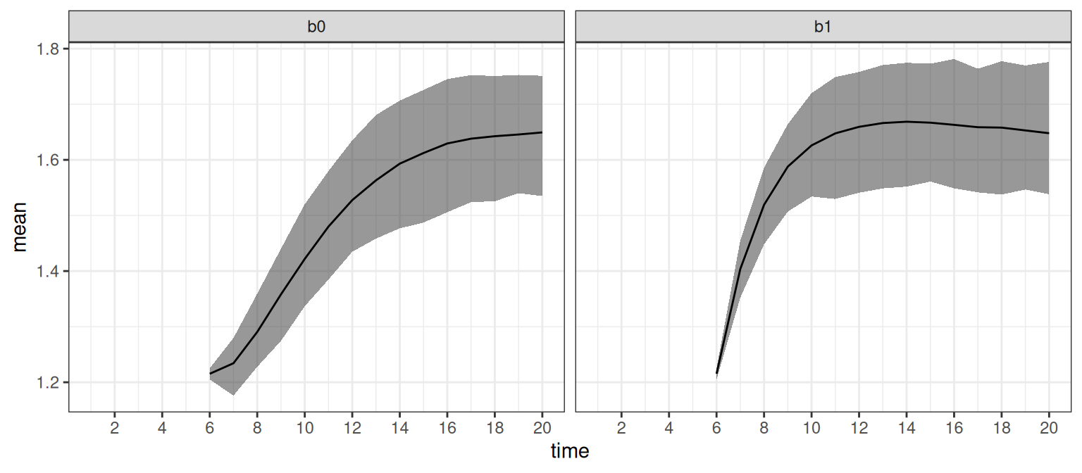
Predictions for the first 5 time points in sumr are NA for all groups by design because our new data supplied to the predict() method for both interventions contained observations for those time points, which is why we set na.rm = TRUE to avoid a warning in the above code. Note that these estimates do indeed coincide with the causal effects (assuming of course that our model is correct), as we can apply the backdoor adjustment formula (Pearl 1995) to obtain the expected causal effect: \[ E(g_t | do(b_5 = x)) = \int E(g_t | b_5 = x, g_5, p_5)P(g_5, p_5)\,dg_5 dp_5, \] where the integral over \(p_5\) should be understood as a sum as \(p_5\) is discrete. In the code above, mean_t is the estimate of this expected value. In addition, we compute an estimate of the difference \[ E(g_t | do(b_5 = 1)) - E(g_t | do(b_5 = 0)), \] to directly compare the effects of the interventions by writing:

sumr_diff <- list(b0 = pred0, b1 = pred1) |>
  bind_rows(.id = "case") |>
  group_by(.draw, time) |>
  summarize(
    mean_t = mean(g_mean[case == "b1"] - g_mean[case == "b0"])
  ) |>
  group_by(time) |>
  summarize(
    mean = mean(mean_t),
    q5 = quantile(mean_t, 0.05, na.rm = TRUE),
    q95 = quantile(mean_t, 0.95, na.rm = TRUE)
  )

We can also plot the difference between the expected causal effects as shown in Figure 4 by running:

ggplot(sumr_diff, aes(time, mean)) +
  geom_ribbon(aes(ymin = q5, ymax = q95), alpha = 0.5) +
  geom_line(na.rm = TRUE) +
  scale_x_continuous(n.breaks = 10)

Figure 4: Difference between the expected causal effects \(E(g_t | do(b_5 = 1)) - E(g_t | do(b_5 = 0))\). The black line shows the posterior mean and the gray area shows a 90% posterior interval.

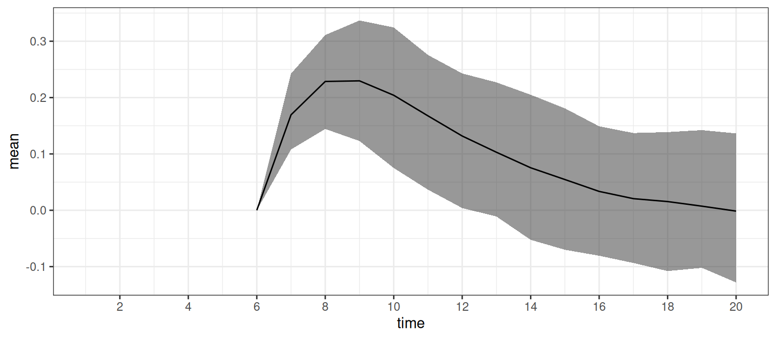
This shows that there is a short-term effect of \(b_5\) on \(g_t\) where the size of the effect diminishes towards zero in time, although the posterior uncertainty is quite large.

4 Model construction

Here we describe the various model components that can be included in the model formulas of the dynamite package. These components are modular and easily combined in any order via a specialized + operator while ensuring that the model formula is well-defined and syntactically valid before estimating the model. The model formula components define the response channels, auxiliary channels, the splines used for time-varying coefficients, correlated random effects, and latent factors.

4.1 Defining response channels

The response channels are defined by combining the channel-specific formulas defined via the function dynamiteformula() for which a shorthand alias obs() is also provided. We will henceforth use this alias for brevity. The function obs() takes three arguments: formula, family, and link which define how the response variable of the channel depends on the covariates in the standard R formula syntax, the family of the response variable as a "character" string, and the link function to use as a "character" string, respectively. The link function specification is optional with each family having a default link. The channel-specific definitions are combined into a single model definition with the + operator of "dynamiteformula" objects. For example, the following formula

dform <- obs(y ~ lag(x), family = "gaussian") +
  obs(x ~ z, family = "poisson")

defines a model with two channels. First, we declare that y is a Gaussian response variable depending on the previous value of x (lag(x)). Next, we add a second channel declaring x as Poisson distributed depending on an exogenous variable z (for which we do not define any distribution). Note that the model formula can be defined without referencing any external data, just like an R formula can. The model formula is an object of class "dynamiteformula" for which the print() method provides a summary of the defined channels, including the response variable names, the channel families and formulas, and other model components:

print(dform)
#>   Family   Formula   
#> y gaussian y ~ lag(x)
#> x poisson  x ~ z

Currently, the package supports the following distributions for the observations:

• Bernoulli ("bernoulli") with logit link.
• Beta ("beta") with logit link, using mean and precision parametrization.
• Binomial ("binomial") with logit link.
• Categorical ("categorical") with a softmax link using the first category as the reference. It is recommended to use Stan version 2.23 or higher which enables the use of the categorical_logit_glm function in the generated Stan code for improved computational performance. See the documentation of categorical_logit_glm in the Stan function reference manual (https://mc-stan.org/users/documentation/) for further information.
• Exponential ("exponential") with log link.
• Gamma ("gamma") with log link, using mean and shape parametrization.
• Gaussian ("gaussian") with identity link, parameterized using mean and standard deviation.
• Multinomial ("multinomial") with a softmax link using the first category as the reference.
• MultivariateGaussian] ("mvgaussian") with identity link for each dimension, parameterized using the mean vector, the standard deviation vector, and the Cholesky decomposition of the correlation matrix.
• Negative binomial ("negbin") with log link, using mean and dispersion parametrization, with an optional known offset variable. See the documentation of the NegBinomial2() function in the Stan function reference manual.
• Ordered ("cumulative") with logit or probit link for ordinal regression using cumulative parametrization for the class probabilities.
• Poisson ("poisson") with log link, with an optional known offset variable.
• Student \(t\) ("student") with identity link, parameterized using location, scale, and degrees of freedom.

There is also a special response variable type "deterministic" which can be used to define deterministic transformations of other variables in the model. This special channel type is explained in greater detail in Section 4.8.

4.2 Lagged responses and covariates

Models in the dynamite package have limited support for contemporaneous dependencies to avoid complex cyclic dependencies that would render the processing of missing data, subsequent predictions, and causal inference challenging or impossible. In other words, the model structure must be acyclic in a sense that there is an order of the response variables such that each response at time \(t\) can be unambiguously defined in this order in terms of responses that have already been defined at time \(t\) or in terms of other variables in the model at time \(t-1\) as formulated in Equation (1). The acyclicity of the model implied by the model formula defined by the user is checked automatically upon construction. To demonstrate, the following formula is valid:

obs(y ~ x, family = "gaussian") +
  obs(x ~ z, family = "poisson")

but the following is not, as y is defined in terms of x, x is defined in terms of z, and z is defined in terms of y, creating a cycle from y to y. This type of model formulation produces an error due to the cyclic definition of the responses:

obs(y ~ x, family = "gaussian") +
  obs(x ~ z, family = "poisson") +
  obs(z ~ y, family = "categorical")
#> Error in `join_dynamiteformulas()`:
#> ! The model must be acyclic.

On the other hand, there are no limitations concerning the dependence of response variables and their previous values or previous values of exogenous covariates, i.e., lags. In the first example of Section 4.1, we used the syntax lag(x), a shorthand for lag(x, k = 1), which defines a first-order lag of the variable x to be used as a covariate. Higher-order lags can also be defined by adjusting the argument k. The argument x of lag() can either be a response variable or an exogenous covariate.

The model component lags() can also be used to quickly add lagged responses as covariates across multiple channels. This component adds a lagged value of each response in the model as a covariate to every channel. For example, calling

obs(y ~ z, family = "gaussian") +
  obs(x ~ z, family = "poisson") +
  lags(k = 1)

would add lag(y, k = 1) and lag(x, k = 1) as covariates of x and y. Therefore, the previous code would produce the same model as writing

obs(y ~ z + lag(y, k = 1) + lag(x, k = 1), family = "gaussian") +
  obs(x ~ z + lag(y, k = 1) + lag(x, k = 1), family = "poisson")

The function lags() can help to simplify the individual model formulas, especially when the model consists of many channels each containing a large number of lags. Just as with the function lag(), the argument k in lags() can be adjusted to add higher-order lags of each response to each channel, but for lags() it can also be a vector so that multiple lags can be added at once. The inclusion of lagged response variables in the model implies that some time points must be considered fixed in the estimation. The number of fixed time points in the model is equal to the highest order lag \(k\) of any observed response variable in the model (defined either via lag() terms or the model component lags()). Lags of exogenous covariates do not affect the number of fixed time points, as such covariates are not modeled.

4.3 Time-varying and time-invariant effects

The formula argument of obs() can also contain a special term varying(), which defines the time-varying part of the model equation. For example, we could write

obs(x ~ z + varying(~ -1 + w), family = "poisson")

to define a model equation with a time-invariant intercept, a time-invariant effect of z, and a time-varying effect of w. We also avoid defining a duplicate intercept by writing -1 within varying() in order to avoid identifiability issues in the model estimation. Alternatively, we could define a time-varying intercept, in which case we would write:

obs(x ~ -1 + z + varying(~ w), family = "poisson")

The part of the formula not wrapped with varying() is assumed to correspond to the time-invariant part of the model, which can alternatively be defined with the special syntax fixed(). This means that the following lines would all produce the same model:

obs(x ~ z + varying(~ -1 + w), family = "poisson")
obs(x ~ -1 + fixed(~ z) + varying(~ -1 + w), family = "poisson")
obs(x ~ fixed(~ z) + varying(~ -1 + w), family = "poisson")

The use of fixed() is therefore optional in the formula. If both time-varying and time-invariant intercepts are defined, the model will default to using a time-varying intercept and an appropriate warning is provided for the user:

obs(y ~ 1 + varying(~1), family = "gaussian")
#> Warning: Both time-constant and time-varying intercept specified:
#> ℹ Defaulting to time-varying intercept.
#>   Family   Formula            
#> y gaussian y ~ 1 + varying(~1)

When defining time-varying effects, we also need to define how their respective regression coefficients depend on time. For this purpose, a splines() component should be added to the model formula, e.g.,

obs(x ~ varying(~ -1 + w), family = "poisson") +
  splines(df = 10)

defines a cubic B-spline with 10 degrees of freedom for the time-varying coefficients, which corresponds to the coefficient of the variable w in this instance. If the model contains multiple time-varying coefficients, the same spline basis is used for all coefficients, with unique spline coefficients and their corresponding random-walk standard deviations for each coefficient. The splines() component constructs the matrix of cardinal B-splines \(B_t\) using the bs() function of the splines package based on the degrees of freedom (df) and the degree of the polynomials used to construct the splines (degree, the default being 3 corresponding to cubic B-splines). It is also possible to switch between centered (the default) and non-centered parametrization (Papaspiliopoulos, Roberts, and Sköld 2007) for the spline coefficients using the noncentered argument of the splines() component. This can affect the sampling efficiency of Stan, depending on the model and the informativeness of the data (M. J. Betancourt and Girolami 2013).

4.4 Group-level random effects

Random effect terms of a channel for each group can be defined using the special term random() within the formula argument of obs(), analogously to varying() and fixed(). By default, all random effects within a group and across all channels are modeled as zero-mean multivariate Gaussian. The optional model component random_spec() can be used to define non-correlated random effects as random_spec(correlated = FALSE). In addition, as with the spline coefficients, it is possible to switch between centered and non-centered (the default) parametrization of the random effects using the noncentered argument of random_spec().

For example, the following code defines a Gaussian response variable x with a time-invariant common effect of z as well as a group-specific intercept and group-specific effect of z.

obs(x ~ z + random(~1 + z), family = "gaussian")

The variable that defines the groups in the data is provided in the call to the model fitting function dynamite() via the group argument as shown in Section 5.

4.5 Latent factors

Instead of common time-varying intercept terms, it is possible to define channel-specific univariate latent factors using the lfactor() model component. Each latent factor is modeled as a spline, with degrees of freedom and spline degree defined via the splines() component (in the case that the model also contains time-varying effects, the same spline basis definition is currently used for both latent factors and time-varying effects). The argument responses of lfactor() defines which channels should contain a latent factor, while argument correlated determines whether the latent factors should be modeled as correlated. Again, users can switch between centered and non-centered parametrizations using the argument noncentered_psi.

In general, dynamic latent factors are not identifiable without imposing some constraints on the factor loadings \(\lambda\) or the latent factor \(\psi\) (see e.g., Bai and Wang 2015), especially in the context of DMPMs and dynamite. In dynamite, these identifiability problems are addressed via internal reparametrization and an additional argument nonzero_lambda which determines whether we assume that the expected value of the factor loadings is zero or not. The theory and thorough experiments regarding the robustness of these identifiability constraints is a work in progress, so some caution should be used regarding the use of the lfactor() component.

4.6 Multivariate channels

While models with more than one channel are multivariate by definition, it is also possible to define individual channels whose responses follow multivariate distributions. In obs(), a multivariate response should be given by specifying the data variables that define its dimensions and combining them with c(). For instance, suppose that we wish to define a multivariate Gaussian channel whose dimensions are given by variables y1, y2, and y3 with a time-invariant effect of x for each dimension. Then we would write:

obs(c(y1, y2, y3) ~ x, family = "mvgaussian")

It is also possible to define a distinct formula for each dimension by separating the dimension-specific definitions with a vertical bar |, for example

obs(c(y1, y2, y3) ~ 1 | x | lag(y1), family = "mvgaussian")

would define no covariates for the first dimension, x as a covariates for the second dimension, and the lagged value of the first dimension as a covariate for the third dimension. The dimension-specific formulas can contain time-invariant and time-varying effects, group-specific random effects, and latent factors, just like univariate channel formulas can.

4.7 Number of trials and offset variables

The special terms trials() and offset() define the number of trials for binomial and multinomial channels, and an offset variable for negative binomial and Poisson channels, respectively. The arguments to these special terms can be exogenous covariates or other response variables of the model, as long as the possible contemporaneous dependencies do not violate the acyclicity of the model as described in Section 4.2. For example, the size of a population could be used as an offset when modeling the prevalence of a disease. Modeling the population size in addition to the prevalence enables future predictions for the prevalence when the future population size is unknown.

Both trials() and offset() terms are added to the formula similar to varying() or random() terms:

obs(y ~ z + trials(n), family = "binomial") +
  obs(x ~ z + offset(w), family = "poisson")

The code above would define a model with a binomial response y with a time-invariant effect of z and the number of trials given by the variable n, and a Poisson response x with a time-invariant effect of z and the variable w as the offset.

4.8 Auxiliary channels

In addition to declaring response variables via obs(), we can also use the function aux() to define auxiliary channels which are deterministic transformations of other variables in the model. Defining these auxiliary variables explicitly instead of defining them implicitly on the right-hand side of the formulas, i.e., by using the “as is” function I(), makes the subsequent prediction steps clearer and allows easier checks of the model validity. Because of this, we do not allow the use of I() in the formula argument of dynamiteformula(). The values of auxiliary variables are computed automatically when fitting the model, and dynamically during prediction, making the use of lagged values and other transformations possible and automatic in prediction as well. An example of a model formula using an auxiliary channel could be

obs(y ~ lag(log1x), family = "gaussian") +
  obs(x ~ z, family = "poisson") +
  aux(numeric(log1x) ~ log(1 + x) | init(0))

For auxiliary channels, the formula declaration via ~ should be understood as mathematical equality or assignment, where the right-hand side provides the defining expression of the variable on the left-hand side. Thus, the example above defines a new auxiliary channel whose response is log1x defined as the logarithm of 1 + x, and assigns it to be of type "numeric". The type declaration is required, because it might not be possible to unambiguously determine the type of the response variable based on its expression alone from the data, especially if the expression contains "factor" type variables. Supported types include "factor", "numeric", "integer", and "logical". A warning is issued to the user if the type declaration is missing from the auxiliary channel definition, and the channel will default to the "numeric" type:

aux(log1x ~ log(1 + x) | init(0))
#> Warning: No type specified for deterministic channel `log1x`:
#> ℹ Assuming type is <numeric>.
#>       Family        Formula                     
#> log1x deterministic log1x ~ log(1 + x) | init(0)

Auxiliary variables can be used directly in the formulas of other channels, just like any other variable. The function aux() does not use the family argument, as the family is automatically set to "deterministic" which is a special channel type of the obs() function. Note that lagged values of deterministic auxiliary channels do not imply fixed time points. Instead, they must be given starting values using one of the two special syntax variants, init() or past() after the main formula separated by the | symbol.

In the example above, because the channel for y contains a lagged value of log1x as a covariate, we also need to supply log1x with a single initial value that determines the value of the lag at the first time point. Here, init(0) defines the initial value of lag(log1x) to be zero for all individuals. In general, if the model contains higher-order lags of an auxiliary channel, then init() can be supplied with a vector initializing each lag.

While init() defines the same starting value to be used for all individuals, an alternative, special syntax past() can be used, which takes an R expression as its argument and computes the starting value for each individual based on that expression. The expression is evaluated in the context of the data supplied to the model fitting function dynamite(). For example, instead of init(0) in the example above, we could write:

obs(y ~ lag(log1x), family = "gaussian") +
  obs(x ~ z, family = "poisson") +
  aux(numeric(log1x) ~ log(1 + x) | past(log(z)))

which defines that the value of lag(log1x) at the first time point is log(z) for each individual, using the value of z in the data to be supplied to compute the actual value of the expression. The special syntax past() can also be used if the model contains higher-order lags of auxiliary responses. In this case, additional observations from the variables bound by the expression given as the argument will simply be used to define the initial values.

4.9 Visualizing the model structure

A plot() method is available for "dynamiteformula" objects that can be used to easily visualize the overall model structure as a DAG. This method can produce either a "ggplot" object of the model plot or a "character" string describing a TikZ (Tantau 2024) code to render the figure in a report, for example. As an illustration, we produce an analogous "ggplot" version of the DAG depicting the multichannel model that was considered in Section 3.2. Figure 5 shows the plots obtained by running the following.

plot(multi_formula)
plot(multi_formula, show_auxiliary = FALSE)

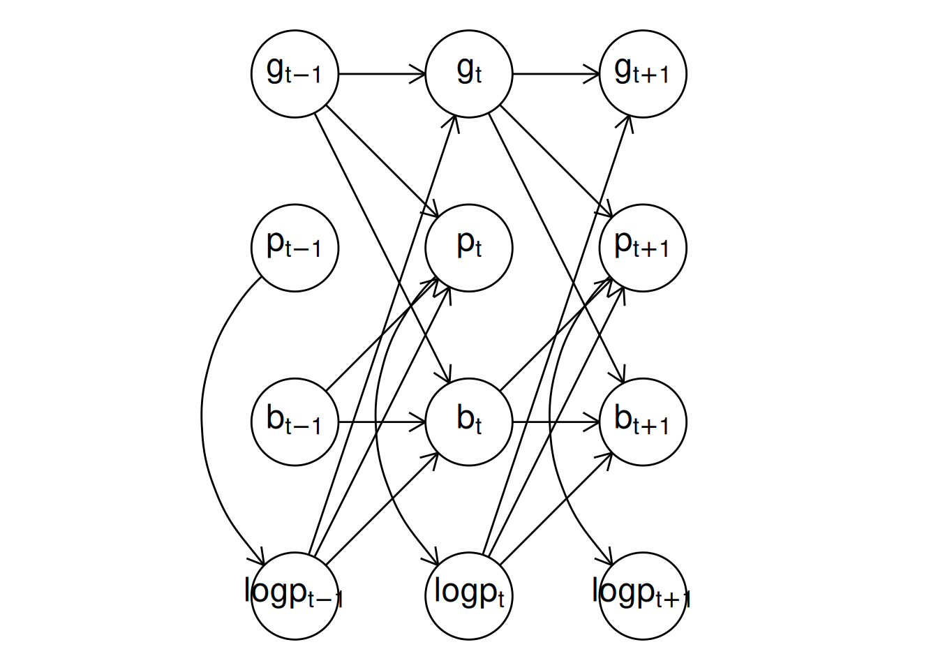
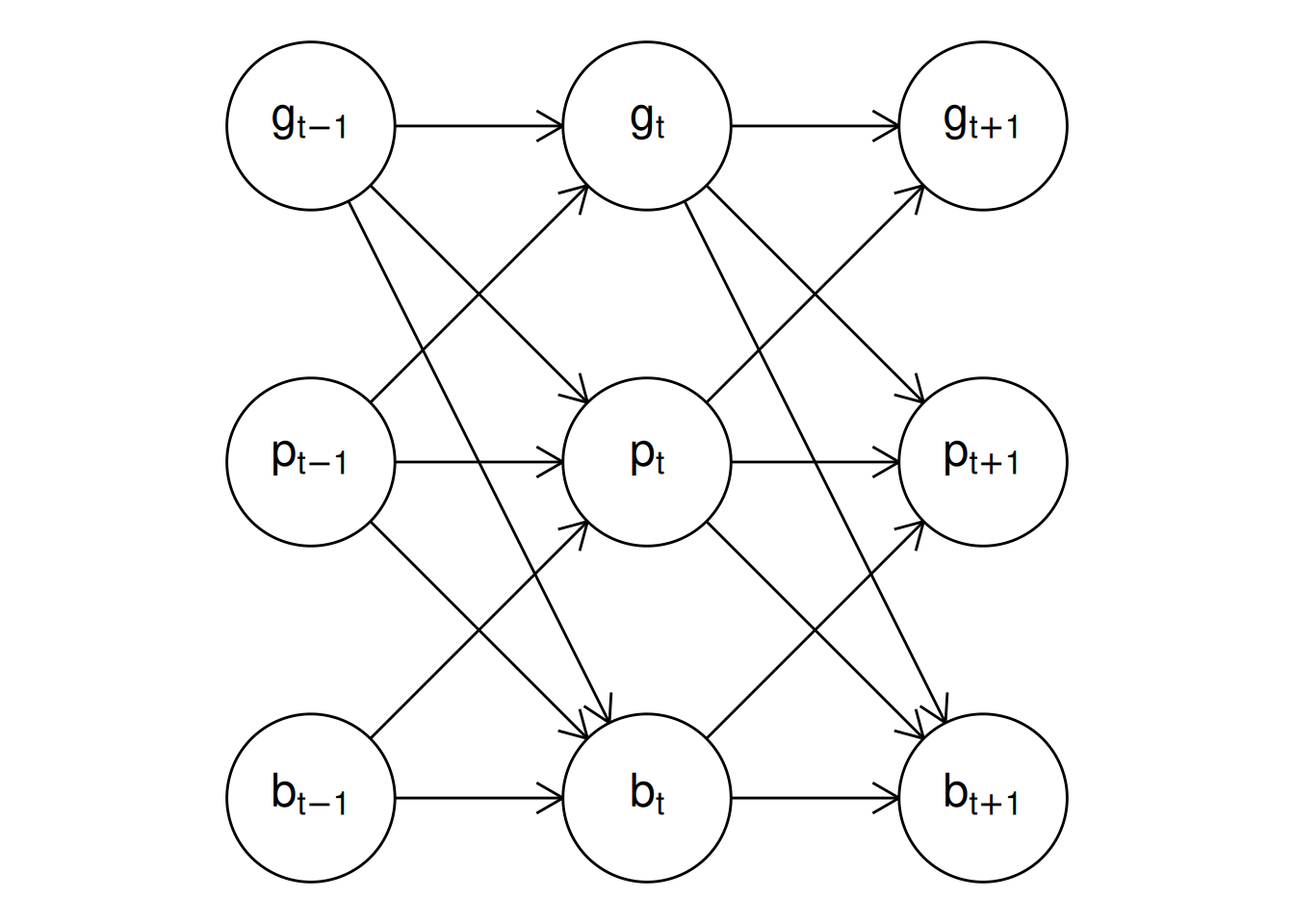
Figure 5: DAGs for the multichannel model created using the plot() method for "dynamitefit" objects. The left panel shows the model structure including the auxiliary channel logp while the right panel shows the model structure where the auxiliary channel is not included. The latter DAG is obtained via a functional projection where the parents of logp become the parents of the children of logp and logp is removed from the graph at each timepoint.

Above, we used the argument show_auxiliary to project out the deterministic auxiliary variable logp from the DAG shown in the right panel of Figure 5, which produces the same DAG as shown in Figure @ref(fig:multichannel_dag). In addition, the argument show_covariates can be used to control whether exogenous covariates should be included in the plot (the default is FALSE hiding covariates). Vertical, horizontal, and diagonal edges that would otherwise pass through vertices are automatically curved in the resulting figure to avoid overlapping with the vertices, but this can still occur with more complicated models.

As demonstrated by Figure 5, mathematical notation is not always rendered ideally in "ggplot" figures. To generate publication-quality figures with vector graphics, the argument tikz is provided. By setting tikz = TRUE, we can obtain the corresponding TikZ code for the figure as follows:

cat(plot(multi_formula, show_auxiliary = FALSE, tikz = TRUE))
#> % Preamble
#> \usepackage{tikz}
#> \usetikzlibrary{positioning, arrows.meta, shapes.geometric}
#> \tikzset{%
#>   semithick,
#>   >={Stealth[width=1.5mm,length=2mm]},
#>   obs/.style 2 args = {
#>     name = #1, circle, draw, inner sep = 8pt, label = center:$#2$
#>   }
#> }
#> % DAG
#> \begin{tikzpicture}
#>   \node [obs = {v1}{g_{t - 1}}] at (-1, 3) {\vphantom{0}};
#>   \node [obs = {v2}{p_{t - 1}}] at (-1, 2) {\vphantom{0}};
#>   \node [obs = {v3}{b_{t - 1}}] at (-1, 1) {\vphantom{0}};
#>   \node [obs = {v4}{g_{t + 1}}] at (1, 3) {\vphantom{0}};
#>   \node [obs = {v5}{p_{t + 1}}] at (1, 2) {\vphantom{0}};
#>   \node [obs = {v6}{b_{t + 1}}] at (1, 1) {\vphantom{0}};
#>   \node [obs = {v7}{g_{t}}] at (0, 3) {\vphantom{0}};
#>   \node [obs = {v8}{p_{t}}] at (0, 2) {\vphantom{0}};
#>   \node [obs = {v9}{b_{t}}] at (0, 1) {\vphantom{0}};
#>   \draw [->] (v1) -- (v7);
#>   \draw [->] (v1) -- (v8);
#>   \draw [->] (v3) -- (v8);
#>   \draw [->] (v3) -- (v9);
#>   \draw [->] (v1) -- (v9);
#>   \draw [->] (v2) -- (v7);
#>   \draw [->] (v2) -- (v8);
#>   \draw [->] (v2) -- (v9);
#>   \draw [->] (v7) -- (v4);
#>   \draw [->] (v7) -- (v5);
#>   \draw [->] (v9) -- (v5);
#>   \draw [->] (v9) -- (v6);
#>   \draw [->] (v7) -- (v6);
#>   \draw [->] (v8) -- (v4);
#>   \draw [->] (v8) -- (v5);
#>   \draw [->] (v8) -- (v6);
#> \end{tikzpicture}

The default style used in the generated TikZ code mimics the style used in Figure 1.

5 Model fitting and posterior inference

To estimate the model, the declared model formula is supplied to the dynamite() function, which has the following arguments:

dynamite(
  dformula, data, time, group = NULL, priors = NULL, backend = "rstan",
  verbose = TRUE, verbose_stan = FALSE, stanc_options = list("O0"),
  threads_per_chain = 1L, grainsize = NULL, custom_stan_model = NULL,
  debug = NULL, ...
)

This function parses the model formula and the data to generate a custom Stan model, which is then compiled and used to simulate the posterior distribution of the model parameters. The first three arguments of the function are mandatory. The first argument dformula is a "dynamiteformula" object that defines the model using the model components described in Section 4. The second argument data is a "data.frame" or a "data.table" object that contains the variables used in the model formula. The third argument time is a column name of data that specifies the unique time points.

The remaining arguments of the function are optional. The group argument is a column name of data that specifies the unique groups (individuals), and when group is NULL we assume that there is only a single group (or individual). The argument priors supplies user-defined priors for the model parameters. The Stan backend can be selected using the backend argument, which accepts either "rstan" (the default) or "cmdstanr". These options correspond to using the rstan and cmdstanr packages for the estimation, respectively. The verbose and verbose_stan arguments control the verbosity of the output from dynamite() and Stan, respectively. Additional C++ compiler options such as the optimization level can be specified with stanc_options when using the "cmdstanr" backend.

While Stan supports between-chain parallelization via the cores and parallel_chains arguments for the "rstan" and "cmdstanr" backends, respectively, it also supports within-chain parallelization. In between-chain parallelization, the computations are split such that a single process is assigned one or more Markov-chains whereas in within-chain parallelization, the computations related to a single Markov chain are split, such as conditionally independent likelihood function evaluations. Both forms of parallelization can be leveraged via dynamite(). For between-chain parallelization, the cores and parallel_chains arguments can be passed directly to the backend sampling function via ... (either rstan::sampling() or the sample() method of the "CmdStanModel" model object). For within-chain parallelization, threaded variants of all likelihood functions have been implemented in dynamite for the reduce-sum functionality of Stan, and the following two arguments are provided: threads_per_chain controls the number of threads to use per chain, and grainsize defines the suggested size of the partial sums (see the Stan manual for further information).

A custom Stan model code can be provided via custom_stan_model, which can be either a "character" string containing the model code or a path to a .stan file that contains the model code. Using this argument will override the automatically generated model code and it is intended for expert users only. Model customization is discussed at greater length in the related package vignette that can be accessed by writing vignette("dynamite_custom", package = "dynamite"). The debug argument can be used for various debugging options (see ?dynamite for further information on these options and other arguments of the function).

The data argument should be supplied in long format, i.e., with \(N \times T\) rows in case of balanced panel data. Acceptable column types of data are "integer", "logical", "double", "character", objects of class "factor", and objects of class "ordered factor". Columns of the "character" type will be converted to "factor" columns. Beyond these standard types, any special classes such as "Date" whose internal storage type is one of the aforementioned types can be used, but these classes will be dropped, and the columns will be converted to their respective storage types. List columns are not supported. The time argument should be a "numeric" or a "factor" column of data. If time is a "factor" column, it will be converted to an "integer" column. Missing values in both response and predictor columns are supported but non-finite values are not. Observations with missing covariate or response values are omitted from the data when the model is fitted.

As an example, the following function call would estimate the model using data in the data frame d, which contains the variables year and id (defining the time-index and group-index variables of the data, respectively). Arguments chains and cores are passed to rstan::sampling() which then uses two parallel Markov chains in the MCMC sampling of the model parameters (as defined by chains = 2 and cores = 2).

dynamite(
  dformula = obs(x ~ varying(~ -1 + w), family = "poisson") +
    splines(df = 10),
  data = d, time = "year", group = "id",
  chains = 2, cores = 2
)

The output of dynamite() is a "dynamitefit" object for which the standard S3 methods such as summary(), plot(), print(), fitted(), and predict() are provided along with various other methods and utility functions which we will describe in the following sections in more detail.

5.1 User-defined priors

The function get_priors() can be used to determine the parameters of the model whose prior distribution can be customized. The function can be applied to an existing model fit object ("dynamitefit") or a model formula object ("dynamiteformula"). The function returns a "data.frame" object, which the user can then manipulate to include their desired priors and subsequently supply to the model fitting function dynamite(). The rationale behind the default prior specifications is discussed in detail in the related package vignette which can be viewed by writing vignette("dynamite_priors", package = "dynamite").

For instance, using the model fit object gaussian_example_fit available in the dynamite package, we have the following priors:

get_priors(gaussian_example_fit)
#>          parameter response             prior      type category
#> 1 sigma_nu_y_alpha        y    normal(0, 3.1)  sigma_nu         
#> 2          alpha_y        y  normal(1.5, 3.1)     alpha         
#> 3      tau_alpha_y        y    normal(0, 3.1) tau_alpha         
#> 4         beta_y_z        y    normal(0, 3.1)      beta         
#> 5        delta_y_x        y    normal(0, 3.1)     delta         
#> 6   delta_y_y_lag1        y    normal(0, 1.8)     delta         
#> 7          tau_y_x        y    normal(0, 3.1)       tau         
#> 8     tau_y_y_lag1        y    normal(0, 1.8)       tau         
#> 9          sigma_y        y exponential(0.65)     sigma

To customize a prior distribution, the user only needs to manipulate the prior column of the desired parameters in this "data.frame" using the appropriate Stan syntax and parametrization. For a categorical response variable, the column category describes which category the parameter is related to. For model parameters of the same type and response, a vectorized form of the corresponding distribution is automatically used in the generated Stan code if applicable. The definitions of the prior distributions are checked for validity before the model fitting process.

5.2 Extracting model fit information

We can obtain a simple model summary with the print() method of objects of class "dynamitefit". For instance, the model fit object gaussian_example_fit gives the following output:

print(gaussian_example_fit)
#> Model:
#>   Family   Formula                                       
#> y gaussian y ~ -1 + z + varying(~x + lag(y)) + random(~1)
#> 
#> Correlated random effects added for response(s): y
#> 
#> Data: gaussian_example (Number of observations: 1450)
#> Grouping variable: id (Number of groups: 50)
#> Time index variable: time (Number of time points: 30)
#> 
#> NUTS sampler diagnostics:
#> 
#> No divergences, saturated max treedepths or low E-BFMIs.
#> 
#> Smallest bulk-ESS: 178 (sigma_y)
#> Smallest tail-ESS: 156 (tau_alpha_y)
#> Largest Rhat: 1.018 (beta_y_z)
#> 
#> Elapsed time (seconds):
#>         warmup sample
#> chain:1  6.313  3.086
#> chain:2  6.472  3.322
#> 
#> Summary statistics of the time- and group-invariant parameters:
#> # A tibble: 6 × 10
#>   variable      mean median      sd     mad     q5   q95  rhat ess_bulk ess_tail
#>   <chr>        <dbl>  <dbl>   <dbl>   <dbl>  <dbl> <dbl> <dbl>    <dbl>    <dbl>
#> 1 beta_y_z    1.97   1.97   0.0112  0.0113  1.95   1.98  1.02      230.     175.
#> 2 sigma_nu_y… 0.0955 0.0940 0.0117  0.0103  0.0791 0.120 1.00      195.     157.
#> 3 sigma_y     0.198  0.198  0.00404 0.00401 0.192  0.205 0.995     178.     188.
#> 4 tau_alpha_y 0.200  0.193  0.0463  0.0440  0.139  0.283 0.999     211.     156.
#> 5 tau_y_x     0.364  0.348  0.0770  0.0746  0.253  0.497 1.01      198.     187.
#> 6 tau_y_y_la… 0.105  0.102  0.0208  0.0195  0.0764 0.140 1.01      231.     186.

By default, the argument full_diagnostics of the print() method is set to FALSE which means that the model diagnostics are computed only for the time-invariant and non-group-specific parameters. Setting this argument to TRUE will compute the diagnostics for all model parameters which can be time-consuming for complex models. Convergence of the MCMC chains and the smallest effective sample sizes of the model parameters can be assessed using the mcmc_diagnostics() method of "dynamitefit" object whose arguments are the model fit object and n, the number of potentially problematic variables to report (default is 3). We refer the reader to (Vehtari et al. 2021) and to the documentation of the rstan::check_hmc_diagnostics() and posterior::default_convergence_measures() functions for detailed information on the diagnostics reported by the mcmc_diagnostics() function.

mcmc_diagnostics(gaussian_example_fit)
#> NUTS sampler diagnostics:
#> 
#> No divergences, saturated max treedepths or low E-BFMIs.
#> 
#> Smallest bulk-ESS values: 
#>                       
#> nu_y_alpha_id16    106
#> alpha_y[28]        118
#> delta_y_y_lag1[14] 118
#> 
#> Smallest tail-ESS values: 
#>                  
#> alpha_y[7]    109
#> alpha_y[14]   111
#> delta_y_x[13] 114
#> 
#> Largest Rhat values: 
#>                     
#> delta_y_x[12]   1.04
#> delta_y_x[8]    1.03
#> nu_y_alpha_id39 1.03

We note that due to CRAN file size restrictions, the number of stored posterior samples in this example "dynamitefit" object is very small, leading to small effective sample sizes. Diagnostics specific to HMC can be extracted with the hmc_diagnostics() method.

A table of posterior draws or summaries of each parameter of the model can be obtained with the methods as.data.frame() and as.data.table() which differ only by their output type ("data.frame" and "data.table"). More specifically, the output of as.data.frame() is a tibble; a tidyverse variant of data frames of class "tbl_df" as defined in the tibble package (Müller and Wickham 2023). These two methods have the following arguments:

as.data.frame.dynamitefit(
  x, keep.rownames, row.names = NULL, optional = FALSE, types = NULL,
  parameters = NULL, responses = NULL, times = NULL, groups = NULL,
  summary = FALSE, probs = c(0.05, 0.95), include_fixed = TRUE, ...
)

Here, x is the "dynamitefit" object and types is a "character" vector that determines the types parameters that will be included in the output. If types is not used, a "character" vector argument parameters can be used to specify exactly which parameters of the model should be included. The argument responses can be used select parameters that are related to specific response channels. For determining suitable options for the arguments types and parameters, methods get_parameter_types() and get_parameter_names() can be used. The arguments times and groups can be used to further restrict the parameters in the output to only include specific time points or groups, respectively. The argument summary determines whether to provide summary statistics (mean, standard deviation, and quantiles selected by the argument probs) of each parameter, or the full posterior draws. The argument include_fixed determines whether to include parameters related to fixed time points in the output (see Section 4.2 for details on fixed time points). The default arguments of the methods keep.rownames, row.names, optional, and ... are ignored for "dynamitefit" objects. All parameter types used in dynamite are described in Table 2.

Table 2: The parameter types used in dynamite.

Parameter type	Description
"alpha"	Intercept terms (time-invariant \(\alpha_{c}\) or time-varying \(\alpha_{c,t}\))
"beta"	Time-invariant regression coefficients \(\beta_c\)
"corr"	Pairwise correlations of multivariate Gaussian responses
"corr_nu"	Pairwise within-group correlations of random effects \(\nu_{c,i}\)
"corr_psi"	Pairwise correlations of the latent factors \(\psi_{c,t}\)
"cutpoint"	Cutpoints for ordinal regression (time-invariant or time-varying)
"delta"	Time-varying regression coefficients \(\delta_{c,t}\)
"kappa"	The contribution of latent factor loadings in the total variation
"lambda"	Latent factor loadings \(\lambda_{c,i}\) of the latent factors \(\psi_{c,t}\)
"nu"	Group-level random effects \(\nu_{c,i}\)
"omega"	Spline coefficients \(\omega_{c,k}\) of the regression coefficients \(\delta_{c,t}\)
"omega_alpha"	Spline coefficients of the time-varying intercepts \(\alpha_{c,t}\)
"omega_psi"	Spline coefficients of the latent factors \(\psi_{c,t}\)
"phi"	Describes various distributional parameters, such as:
	the dispersion parameter of the negative binomial distribution,
	the shape parameter of the gamma distribution,
	the precision parameter of the beta distribution,
	the degrees of freedom of the Student \(t\) distribution.
"psi"	Latent factors \(\psi_{c,t}\)
"sigma"	Standard deviations of (multivariate) Gaussian responses
"sigma_lambda"	Standard deviations of the latent factor loadings \(\lambda_{c,i}\)
"sigma_nu"	Standard deviations of the random effects \(\nu_{c,i}\)
"tau"	Standard deviations \(\tau_{c,k}\) of \(\omega_{c,k,d}\)
"tau_alpha"	Standard deviations of the spline coefficients of \(\alpha_{c,t}\)
"tau_psi"	Standard deviations of the spline coefficients of \(\psi_{c,t}\)
"zeta"	Total variation of latent factors, i.e., \(\sigma_\lambda + \tau_\psi\)

For instance, we can extract the posterior summary of the time-invariant regression coefficients (types = "beta") for the response variable y in the gaussian_example_fit object by writing:

as.data.frame(
  gaussian_example_fit,
  responses = "y", types = "beta", summary = TRUE
)
#> # A tibble: 1 × 10
#>   parameter  mean     sd    q5   q95  time group category response type 
#>   <chr>     <dbl>  <dbl> <dbl> <dbl> <int> <int> <chr>    <chr>    <chr>
#> 1 beta_y_z   1.97 0.0112  1.95  1.98    NA    NA NA       y        beta

For "dynamitefit" objects, the summary() method is a shortcut for as.data.frame(summary = TRUE).

The generated Stan code of the model can be extracted with the method get_code() as a "character" string. This feature is geared towards advanced users who may for example need to make slight modifications to the generated code in order to adapt the model to a specific scenario that cannot be accomplished with the dynamite model syntax. The generated code also contains helpful annotations describing the model blocks, parameters, and complicated code sections. Using the argument blocks, we can extract only specific blocks of the full model code. To illustrate, we extract the parameters block of the gaussian_example_fit model code as the full model code is too large to display.

cat(get_code(gaussian_example_fit, blocks = "parameters"))
#> parameters {
#>   // Random group-level effects
#>   vector<lower=0>[M] sigma_nu; // standard deviations of random effects
#>   matrix[N, M] nu_raw;
#>   vector[K_fixed_y] beta_y; // Fixed coefficients
#>   matrix[K_varying_y, D] omega_y; // Spline coefficients
#>   vector<lower=0>[K_varying_y] tau_y; // SDs for the random walks
#>   real a_y; // Mean of the first time point
#>   row_vector[D - 1] omega_raw_alpha_y; // Coefficients for alpha
#>   real<lower=0> tau_alpha_y; // SD for the random walk
#>   real<lower=0> sigma_y; // SD of the normal distribution
#> }

Conversely, a customized Stan model code can be supplied to dynamite() using the custom_stan_model argument.

5.3 Visualizing the posterior distributions

The plot() method for "dynamitefit" objects can be used to obtain plots of various types of the model fit using the ggplot2 package to produce the plots. This method has the following arguments:

plot.dynamitefit(
  x, plot_type = c("default", "trace", "dag"), types = NULL,
  parameters = NULL, responses = NULL, groups = NULL, times = NULL,
  level = 0.05, alpha = 0.5, facet = TRUE, scales = c("fixed", "free"),
  n_params = NULL, ...
)

The arguments type, parameters, responses, groups and times are analogous to those of the as.data.frame() method for selecting which parameters should be plotted. Arguments level, alpha, facet and scales control the visual aspects of the plot: level defines the plotted posterior intervals as 100 * (1 - 2 * level) % intervals, alpha is the opacity level for ggplot2::geom_ribbon() for plotting posterior intervals, facet determines whether time-invariant parameters should be plotted together (FALSE) or separately using ggplot2::facet_wrap() (TRUE), and scales selects whether the vertical axis of different parameters should be the same ("fixed") or allowed to vary between parameters ("free"). Finally, n_params controls the maximum number of parameters of each type to plot. By default, the number of parameters is limited to prevent accidental plots with a large number of parameters that may take an excessively long time to render. Next, we showcase some example plots and the different plot types that are available via the plot_type argument.

For instance, Figure 6 shows the posterior means and posterior intervals of the time-varying intercept (type "alpha") and time-varying regression coefficients (type "delta") in the gaussian_example_fit model (using the "default" option of the plot_type argument by default).

plot(
  gaussian_example_fit,
  types = c("alpha", "delta"), scales = "free"
) +
  labs(title = "")

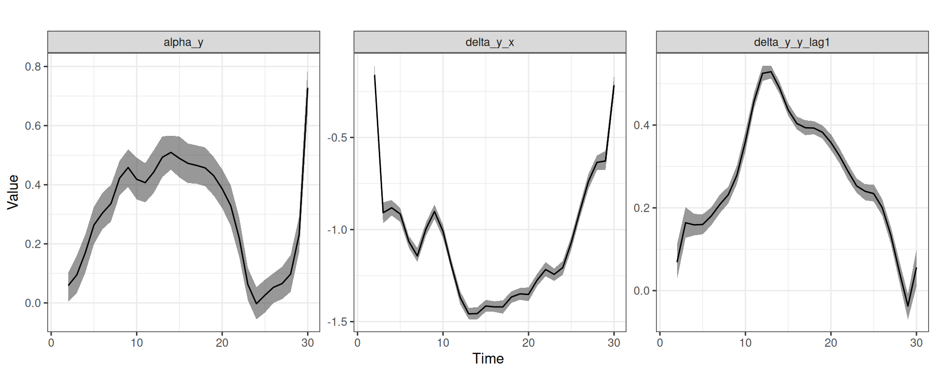
Figure 6: Posterior means (black lines) and 90% posterior intervals (gray areas) for the time-varying coefficients for the response variable y in the gaussian_example_fit model. The panels from left to right show the time-varying intercept for y, the time-varying effect of x on y, and the time-varying effect of lag(y) (the previous time-point) on y.

While plot_type = "default" produces plots such as Figure @ref(fig:parameter_posterior_plot), using plot_type = "trace" instead provides the marginal posterior densities and traceplots of the MCMC chains, as shown in Figure @ref(fig:gaussian_trace) where we also select the time-invariant regression coefficients of the model to be plotted.

plot(gaussian_example_fit, plot_type = "trace", types = "beta")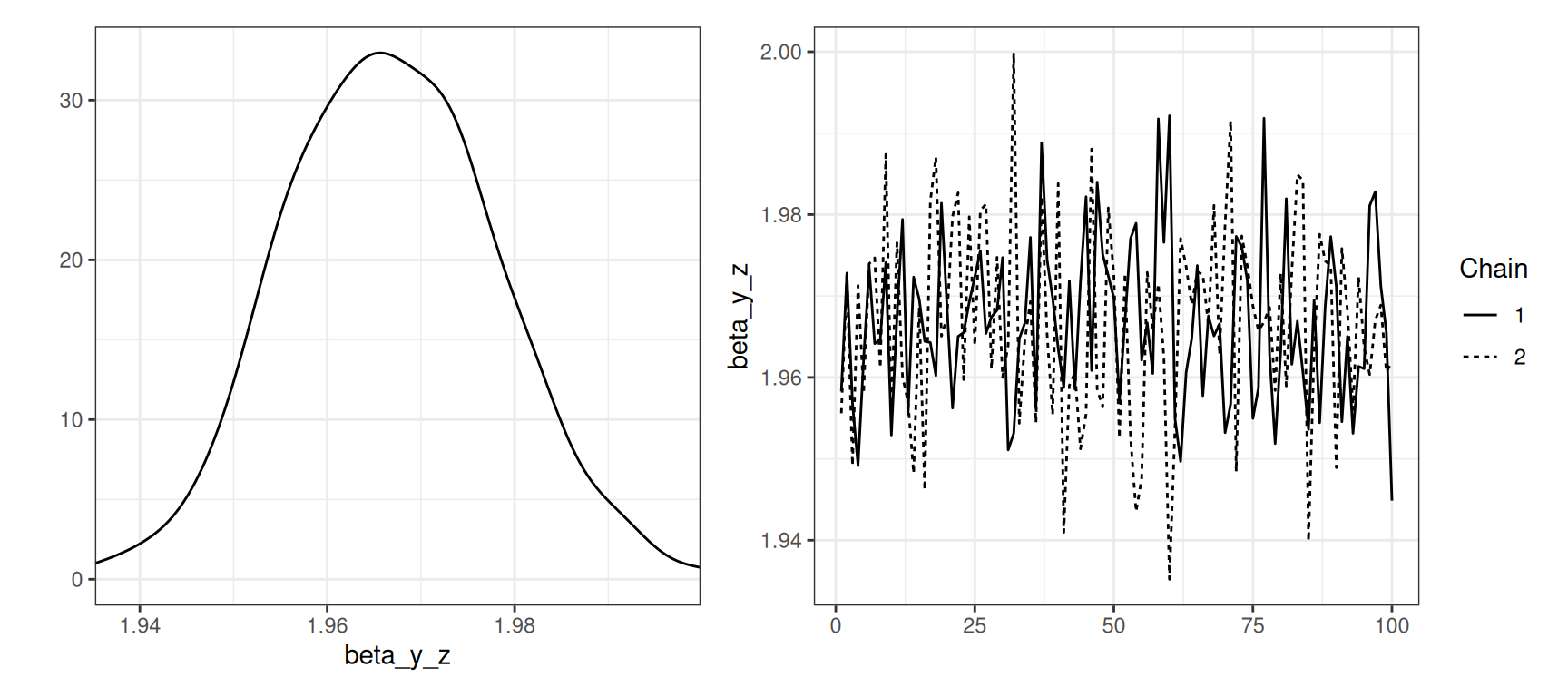

Figure 7: Marginal posterior density and traceplot of the MCMC chains of the time-invariant regression coefficient beta_y_z of z for the response variable y in the gaussian_example_fit model.

The third option plot_type = "dag" can be used to visualize the structure of the model as a DAG as shown in Figure 5 and described in Section 4.9.

5.4 Missing data and multiple imputation

Panel data often contains missing observations for various reasons. A common approach in a Bayesian setting is to treat missing observations as additional unknown parameters, and to sample them along with the model parameters during MCMC. However, the MCMC sampling in dynamite is based on Stan’s variant of the gradient-based NUTS algorithm (Hoffman and Gelman 2014; M. Betancourt 2018), which cannot be used to sample discrete variables such as missing count data. Therefore, the default behavior in dynamite is to use a complete-case approach which is unbiased when data are missing completely at random as well as in certain other specific settings (van Buuren 2018). As an alternative to complete-case analysis with dynamite(), the function dynamice() first performs multiple imputation using the imputation algorithms of the mice package (van Buuren and Groothuis-Oudshoorn 2011), runs MCMC on each imputed sample, and combines the posterior samples of each run, as suggested for example in (Gelman et al. 2013).

The dynamice() function has all of the arguments of dynamite() with some additions. The argument mice_args is a "list" that can be used to provide arguments to the underlying imputation function mice() of the mice package. Format of the data during imputation can be selected with the impute_format argument that accepts either "wide" or "long". Data in wide format will have one group per row (with observations at different time points in different columns) while data in long format corresponds to the standard data format of dynamite() described in Section 5. Argument keep_imputed is a "logical" value can be used to select whether the imputed data sets should be included in the return object of dynamice(). If TRUE, the imputed data sets will be found in the imputed field of the returned "dynamitefit" object. All of the methods for "dynamitefit" objects are available also for model fits obtained from dynamice(), but it should be noted that convergence measures and effective samples sizes such as those reported by mcmc_diagnostics() may be unreliable for such model fits.

6 Prediction

The dynamite package provides a comprehensive set of features for obtaining predictions based on the posterior distribution of the model parameters. The package supports the imputation of missing exogenous covariate values (via last observation carried forward or next observation carried backward), aggregated and individual-level predictions, and various methods to account for new levels of the group variable for random effects. Counterfactual predictions can also be obtained which enables the study of causal effects and other intricate causal quantities. It should be noted that the predictions do not directly support forecasting as there is no unambiguous way to define how the splines for the time-varying regression coefficients should behave outside of the observed time points. However, such predictions can be obtained by augmenting the original data with missing values for future time points. Furthermore, the package can be used to generate data from a DMPM without an existing model fit by first specifying the values of the model parameters and the fixed covariates (see the package vignette on data simulation for further information: vignette("dynamite_simulation", package = "dynamite")).

The predict() method for "dynamitefit" objects can be used to obtain predictions from the posterior predictive distribution. This function has the following arguments:

predict.dynamitefit(
  object, newdata = NULL, type = c("response", "mean", "link"),
  funs = list(), impute = c("none", "locf", "nocb"),
  new_levels = c("none", "bootstrap", "gaussian", "original"),
  global_fixed = FALSE, n_draws = NULL, thin = 1,
  expand = TRUE, df = TRUE, ...
)

We will only explain the most important arguments of this method and refer the reader to the package documentation for more information. The first argument object is the "dynamitefit" object that the predictions will be based on. The argument newdata can be used to define the groups, time points, and covariate values that the predictions should be computed for. If newdata is NULL, predictions will be computed for the original data supplied to the dynamite() function when the model was fitted from the first non-fixed time point onward. The type argument selects the type of computed predictions. By default, type = "response" returns the individual-level simulated predictions for the response variables of the model. Options "link" and "mean" return the linear predictor values and the expected values of the posterior predictive distribution, respectively. The argument n_draws controls the number of posterior draws to be used for prediction. By default, all draws are used. Alternatively, the argument thin can be used to select every thinth posterior draw to be used for the prediction task.

For example, we can obtain posterior predictive samples for the first 4 groups in the gaussian_example dataset using the corresponding model fit object gaussian_example_fit with the first 50 posterior draws. The predictions are shown in Figure 8 and can be obtained as follows:

pred <- predict(gaussian_example_fit, n_draws = 50)
pred |>
  dplyr::filter(id < 5) |>
  ggplot(aes(time, y_new, group = .draw)) +
  geom_line(alpha = 0.5) +
  geom_line(aes(y = y), colour = "tomato") +
  facet_wrap(~ id)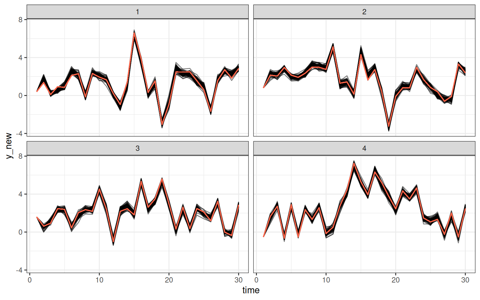

Figure 8: Posterior predictive samples for the first 4 groups of the gaussian_example data. Lines in red represent the observed values.

The fitted() method is also provided for "dynamitefit" objects. In contrast to multi-step predictions of predict(), this function computes expected values of the posterior predictive distributions at each time point conditional on the original observations.

We note that the multi-step predictions contain not only the parameter uncertainty but also the inherent aleatoric (stochastic) uncertainty of the trajectories. The Monte Carlo variation due to the finite number of posterior samples can be reduced by increasing the number of iterations or chains of the MCMC run (as with any posterior summaries) or by combining samples from multiple predict() calls in case the Monte Carlo error is mostly due to the trajectory simulation.

6.1 Aggregated predictions and memory conservation

For large datasets and complicated models, obtaining individual-level predictions can be memory-intensive. For example, data with 100 groups, 100 time points, a categorical response with 4 categories, and 1000 posterior draws would result in 40 million elements. A simple way to reduce memory usage is to set the argument expand of predict() to FALSE (the default is TRUE). Disabling this argument separates the simulated values from the fixed covariates in the model into two "data.table" objects in the output, called simulated and observed, which are then returned as a "list" object. This optimization is always carried out internally, meaning that the value of the expand argument only affects the returned output.

To further reduce memory usage, the argument funs can be used to obtain aggregated predictions instead of the full individual-level predictions for each time point. This argument accepts a named list of lists of named functions for each response channel of the model, where the supplied functions are then applied over the individuals. The resulting columns in the output are named based on the function names and the response variables. The expand argument is automatically set to FALSE when using the funs argument. For example, we could compute the mean and standard deviation of the predictions for the response variable y in the gaussian_example dataset at each time point as follows:

pred_funs <- predict(
  gaussian_example_fit,
  funs = list(y = list(mean = mean, sd = sd))
)
head(pred_funs$simulated)
#>     mean_y      sd_y time .draw
#> 1       NA        NA    1     1
#> 2 1.504474 0.8527229    2     1
#> 3 1.705757 1.3061120    3     1
#> 4 1.722222 1.2155877    4     1
#> 5 2.121926 1.2646230    5     1
#> 6 2.186567 1.3738596    6     1

The reduction in memory usage compared to the full individual-level predictions is rather substantial even in this simple scenario:

library("pryr")
pred_full <- predict(gaussian_example_fit)
object_size(pred_full)
#> 12.00 MB
object_size(pred_funs)
#> 188.34 kB

The funs argument can also be used to aggregate the expected values of the posterior predictive distribution with type = "mean":

pred_funs_mean <- predict(
  gaussian_example_fit,
  type = "mean",
  funs = list(y = list(mean = mean, sd = sd))
)
head(pred_funs_mean$simulated)
#>     mean_y      sd_y time .draw
#> 1       NA        NA    1     1
#> 2 1.512491 0.8425512    2     1
#> 3 1.720646 1.3097006    3     1
#> 4 1.719707 1.1955273    4     1
#> 5 2.099282 1.2462898    5     1
#> 6 2.187195 1.3636075    6     1

7 Summary

In this vignette, we presented the dynamite package for Bayesian inference of DMPMs. The package provides a user-friendly interface for model construction, estimation, prediction, posterior inference, and visualization with extensive and detailed documentation of its features. The package has been designed to be as general as possible by supporting multivariate models, many response variable distributions, custom prior distributions, and common model features such as time-varying effects and group-specific random effects. The package design also aims for high performance in model estimation by employing Stan and in general-purpose data manipulation by using data.table which is especially reflected in prediction. For advanced users, the Stan code generated by dynamite can be extracted and adapted to user-specific scenarios.

In the future, we plan to extend the capabilities of dynamite by adding support for more distributions. Some distributions in Stan also lack efficient likelihood function variants, such as the Bernoulli distribution, which will likely become available in the future and will be subsequently implemented in dynamite as well.

References

Allison, Paul D. 2009. Fixed Effects Regression Models. SAGE Publications. https://doi.org/10.4135/9781412993869.

Allison, Paul D., Richard Williams, and Enrique Moral-Benito. 2017. “Maximum Likelihood for Cross-Lagged Panel Models with Fixed Effects.” Socius 3. https://doi.org/10.1177/2378023117710578.

Arellano, Manuel, and Stephen Bond. 1991. “Some Tests of Specification for Panel Data: Monte Carlo Evidence and an Application to Employment Equations.” The Review of Economic Studies 58 (2): 277–97. https://doi.org/10.2307/2297968.

Asparouhov, Tihomir, Ellen L. Hamaker, and Bengt Muthén. 2018. “Dynamic Structural Equation Models.” Structural Equation Modeling: A Multidisciplinary Journal 25 (3): 359–88. https://doi.org/10.1080/10705511.2017.1406803.

Bai, Jushan, and Peng Wang. 2015. “Identification and Bayesian Estimation of Dynamic Factor Models.” Journal of Business & Economic Statistics 33 (2): 221–40. https://doi.org/10.1080/07350015.2014.941467.

Barrett, Tyson, Matt Dowle, Arun Srinivasan, Jan Gorecki, Michael Chirico, and Toby Hocking. 2024. data.table: Extension of ‘Data.frame‘. https://CRAN.R-project.org/package=data.table.

Bates, Douglas, Martin Mächler, Ben Bolker, and Steve Walker. 2015. “Fitting Linear Mixed-Effects Models Using lme4.” Journal of Statistical Software 67 (1): 1–48. https://doi.org/10.18637/jss.v067.i01.

Bergé, Laurent. 2018. “Efficient Estimation of Maximum Likelihood Models with Multiple Fixed-Effects: The R Package FENmlm.” CREA Discussion Papers, no. 13.

Betancourt, M. J., and Mark Girolami. 2013. “Hamiltonian Monte Carlo for Hierarchical Models.” https://doi.org/10.48550/arXiv.1312.0906.

Betancourt, Michael. 2018. “A Conceptual Introduction to Hamiltonian Monte Carlo.” https://doi.org/10.48550/arXiv.1701.02434.

Bollen, Kenneth A., and Jennie E. Brand. 2010. “A General Panel Model with Random and Fixed Effects: A Structural Equations Approach.” Social Forces 89 (1): 1–34. https://doi.org/10.1353/sof.2010.0072.

Brodersen, Kay H., Fabian Gallusser, Jim Koehler, Nicolas Remy, and Steven L. Scott. 2014. “Inferring Causal Impact Using Bayesian Structural Time-Series Models.” The Annals of Applied Statistics 9 (1): 247–74. https://doi.org/10.1214/14-AOAS788.

Bürkner, Paul-Christian. 2018. “Advanced Bayesian Multilevel Modeling with the R Package brms.” The R Journal 10 (1): 395–411. https://doi.org/10.32614/RJ-2018-017.

Bürkner, Paul-Christian, Jonah Gabry, Matthew Kay, and Aki Vehtari. 2023. posterior: Tools for Working with Posterior Distributions. https://mc-stan.org/posterior/.

Casas, Isabel, and Rubén Fernández-Casal. 2022. “tvReg: Time-Varying Coefficients in Multi-Equation Regression in R.” The R Journal 14: 79–100. https://doi.org/10.32614/RJ-2022-002.

Chow, Sy-Miin, Moon-ho Ringo Ho, Ellen L. Hamaker, and Conor V. Dolan. 2010. “Equivalence and Differences Between Structural Equation Modeling and State-Space Modeling Techniques.” Structural Equation Modeling: A Multidisciplinary Journal 17: 303–32. https://doi.org/10.1080/10705511003661553.

Cohen, Alma, and Liran Einav. 2003. “The Effects of Mandatory Seat Belt Laws on Driving Behavior and Traffic Fatalities.” Review of Economics and Statistics 85 (4): 828–43. https://doi.org/10.2139/ssrn.293582.

Croissant, Yves, and Giovanni Millo. 2008. “Panel Data Econometrics in R: The plm Package.” Journal of Statistical Software 27 (2): 1–43. https://doi.org/10.18637/jss.v027.i02.

———. 2022. pder: Panel Data Econometrics with R. https://CRAN.R-project.org/package=pder.

Durbin, James, and Siem Jan Koopman. 2012. Time Series Analysis by State Space Methods. 2nd ed. New York: Oxford University Press.

Dziak, John J., Donna L. Coffman, Runze Li, Kaylee Litson, and Yajnaseni Chakraborti. 2021. tvem: Time-Varying Effect Models. https://CRAN.R-project.org/package=tvem.

Eubank, R. L., Chunfeng Huang, Y. Muñoz Maldonado, Naisyin Wang, Suojin Wang, and R. J. Buchanan. 2004. “Smoothing Spline Estimation in Varying-Coefficient Models.” Journal of the Royal Statistical Society B 66 (3): 653–67.

Gabry, Jonah, and Rok Češnovar. 2023. cmdstanr: R Interface to CmdStan.

Gelman, Andrew, John B. Carlin, Hal S. Stern, and Donald B. Rubin. 2013. Bayesian Data Analysis. 3rd ed. Chapman; Hall/CRC.

Halekoh, Ulrich, Søren Højsgaard, and Jun Yan. 2006. “The R Package geepack for Generalized Estimating Equations.” Journal of Statistical Software 15/2: 1–11. https://doi.org/10.18637/jss.v015.i02.

Hamaker, Ellen L, Rebecca M Kuiper, and Raoul PPP Grasman. 2015. “A Critique of the Cross-Lagged Panel Model.” Psychological Methods 20 (1): 102. https://doi.org/10.1037/a0038889.

Harvey, A. C., and G. D. A. Phillips. 1982. “The Estimation of Regression Models with Time-Varying Parameters.” In Games, Economic Dynamics, and Time Series Analysis, edited by M. Deistler, E. Fürst, and G. Schwödiauer, 306–21. Physica, Heidelberg. https://doi.org/10.1007/978-3-662-41533-7_18.

Hastie, Trevor, and Robert Tibshirani. 1993. “Varying-Coefficient Models.” Journal of the Royal Statistical Society B 55 (4): 757–96. https://doi.org/10.1111/j.2517-6161.1993.tb01939.x.

Hayakawa, Kazuhiko, and Jie Hou. 2019. “Estimation of Time-Varying Coefficient Dynamic Panel Data Models.” Communications in Statistics - Theory and Methods 48 (13): 3311–24. https://doi.org/10.1080/03610926.2018.1476704.

Helske, Jouni. 2017. “KFAS: Exponential Family State Space Models in R.” Journal of Statistical Software 78 (10): 1–39. https://doi.org/10.18637/jss.v078.i10.

———. 2022. “Efficient Bayesian Generalized Linear Models with Time-Varying Coefficients: The walker Package in R.” SoftwareX 18: 101016. https://doi.org/10.1016/j.softx.2022.101016.

Helske, Jouni, and Santtu Tikka. 2024. “Estimating Causal Effects from Panel Data with Dynamic Multivariate Panel Models.” Advances in Life Course Research 60: 100617. https://doi.org/https://doi.org/10.1016/j.alcr.2024.100617.

Helske, Jouni, and Matti Vihola. 2021. “bssm: Bayesian Inference of Non-Linear and Non-Gaussian State Space Models in R.” The R Journal 13 (2): 578–89. https://doi.org/10.32614/RJ-2021-103.

Hoffman, Matthew D, and Andrew Gelman. 2014. “The No-U-Turn Sampler: Adaptively Setting Path Lengths in Hamiltonian Monte Carlo.” Journal of Machine Learning Research 15 (47): 1593–623. http://jmlr.org/papers/v15/hoffman14a.html.

King, Aaron A., Dao Nguyen, and Edward L. Ionides. 2016. “Statistical Inference for Partially Observed Markov Processes via the R Package pomp.” Journal of Statistical Software 69 (12): 1–43. https://doi.org/10.18637/jss.v069.i12.

Knaus, Peter, Angela Bitto-Nemling, Annalisa Cadonna, and Sylvia Frühwirth-Schnatter. 2021. “Shrinkage in the Time-Varying Parameter Model Framework Using the R Package shrinkTVP.” Journal of Statistical Software 100: 1–32. https://doi.org/10.18637/jss.v100.i13.

Lang, Stefan, and Andreas Brezger. 2004. “Bayesian P-Splines.” Journal of Computational and Graphical Statistics 13 (1): 183–212. https://doi.org/10.1198/1061860043010.

Long, Jacob A. 2020. panelr: Regression Models and Utilities for Repeated Measures and Panel Data. https://cran.r-project.org/package=panelr.

Mulder, Jeroen D., and Ellen L. Hamaker. 2021. “Three Extensions of the Random Intercept Cross-Lagged Panel Model.” Structural Equation Modeling: A Multidisciplinary Journal 28 (4): 638–48. https://doi.org/10.1080/10705511.2020.1784738.

Müller, Kirill, and Hadley Wickham. 2023. tibble: Simple Data Frames. https://CRAN.R-project.org/package=tibble.

Neal, Radford M. 2011. “MCMC Using Hamiltonian Dynamics.” In Handbook of Markov Chain Monte Carlo, edited by Steve Brooks, Andrew Gelman, Galin Jones, and Xiao-Li Meng. Chapman; Hall/CRC. https://doi.org/10.1201/b10905.

Ou, Lu, Michael D. Hunter, and Sy-Miin Chow. 2019. “What’s for dynr: A Package for Linear and Nonlinear Dynamic Modeling in R.” The R Journal 11 (1): 91–111. https://doi.org/10.32614/RJ-2019-012.

Papaspiliopoulos, Omiros, Gareth O. Roberts, and Martin Sköld. 2007. “A General Framework for the Parametrization of Hierarchical Models.” Statistical Science 22 (1): 59–73. https://doi.org/10.1214/088342307000000014.

Papastamoulis, Panagiotis. 2016. “label.switching: An R Package for Dealing with the Label Switching Problem in MCMC Outputs.” Journal of Statistical Software, Code Snippets 69 (1): 1–24. https://doi.org/10.18637/jss.v069.c01.

Pearl, Judea. 1995. “Causal Diagrams for Empirical Research.” Biometrika 82 (4): 669–88. https://doi.org/10.1093/biomet/82.4.669.

———. 2009. Causality: Models, Reasoning, and Inference. 2nd ed. Cambridge University Press.

R Core Team. 2023. R: A Language and Environment for Statistical Computing. Vienna, Austria: R Foundation for Statistical Computing. https://www.R-project.org/.

Rosseel, Yves. 2012. “lavaan: An R Package for Structural Equation Modeling.” Journal of Statistical Software 48 (2): 1–36. https://doi.org/10.18637/jss.v048.i02.

Sallas, William M., and David A. Harville. 1981. “Best Linear Recursive Estimation for Mixed Linear Models.” Journal of the American Statistical Association 76 (376): 860–69. https://doi.org/10.1080/01621459.1981.10477734.

Stan Development Team. 2024a. RStan: The R Interface to Stan. https://mc-stan.org/.

———. 2024b. Stan Modeling Language Users Guide and Reference Manual. https://mc-stan.org/.

Sun, Yiguo, Raymond J Carroll, and Dingding Li. 2009. “Semiparametric Estimation of Fixed-Effects Panel Data Varying Coefficient Models.” In Nonparametric Econometric Methods, 101–29. Advances in Econometrics. Emerald Group Publishing Limited. https://doi.org/10.1108/S0731-9053(2009)0000025006.

Tantau, Till. 2024. The TikZ and PGF Packages: Manual for Version 3.1.10. https://github.com/pgf-tikz/pgf.

Tikka, Santtu, and Jouni Helske. 2024a. “dynamite: An R Package for Dynamic Multivariate Panel Models.” https://arxiv.org/abs/2302.01607.

———. 2024b. dynamite: Bayesian Modeling and Causal Inference for Multivariate Longitudinal Data. https://github.com/ropensci/dynamite.

van Buuren, Stef. 2018. Flexible Imputation of Missing Data. 2nd ed. Chapman; Hall/CRC. https://doi.org/10.1201/9780429492259.

van Buuren, Stef, and Karin Groothuis-Oudshoorn. 2011. “mice: Multivariate Imputation by Chained Equations in R.” Journal of Statistical Software 45 (3): 1–67. https://doi.org/10.18637/jss.v045.i03.

Vehtari, Aki, Jonah Gabry, Mans Magnusson, Yuling Yao, Paul-Christian Bürkner, Topi Paananen, and Andrew Gelman. 2022. loo: Efficient Leave-One-Out Cross-Validation and WAIC for Bayesian Models. https://mc-stan.org/loo/.

Vehtari, Aki, Andrew Gelman, Daniel Simpson, Bob Carpenter, and Paul-Christian Bürkner. 2021. “Rank-Normalization, Folding, and Localization: An Improved \(\widehat{R}\) for Assessing Convergence of MCMC (with Discussion).” Bayesian Analysis 16 (2): 667–718. https://doi.org/https://doi.org/10.1214/20-BA1221.

Wickham, Hadley. 2016. ggplot2: Elegant Graphics for Data Analysis. Springer-Verlag. https://ggplot2.tidyverse.org.

———. 2023. pryr: Tools for Computing on the Language. https://CRAN.R-project.org/package=pryr.

Wickham, Hadley, Romain François, Lionel Henry, Kirill Müller, and Davis Vaughan. 2023. dplyr: A Grammar of Data Manipulation. https://CRAN.R-project.org/package=dplyr.

Wood, Simon N. 2020. “Inference and Computation with Generalized Additive Models and Their Extensions.” TEST 29 (2): 307–39. https://doi.org/10.1007/s11749-020-00711-5.

Wooldridge, Jeffrey M. 2010. Econometric Analysis of Cross Section and Panel Data. MIT Press.

Zyphur, Michael J., Paul D. Allison, Louis Tay, Manuel C. Voelkle, Kristopher J. Preacher, Zhen Zhang, Ellen L. Hamaker, et al. 2020. “From Data to Causes I: Building a General Cross-Lagged Panel Model (GCLM).” Organizational Research Methods 23 (4): 651–87. https://doi.org/10.1177/1094428119847278.

Appendix

A Details on latent factors

Latent factor models with product terms \(\lambda_i\psi_t\) are known to suffer from identifiability issues. For example, it is possible to multiply each \(\lambda_i\) by some constant \(c\) while simultaneously multiplying \(\psi_i, t=1,\ldots, T\) with the reciprocal of the same constant, leading to the same likelihood value as the original model. In case of multiple latent factors and (vector) autoregressive process on \(\psi_t\), discuss two alternative identifiability constraints, which in our single factor model translate to fixing \(\lambda_i = 1\) for some \(i\), or constraining \(\lambda_i > 0\) for some \(i\), with an additional constraint that the standard deviation of the noise term of \(\psi_t\) is 1. In both cases, we need to decide which individual is used as a reference for the constrained \(\lambda_i\). This choice can lead to computational issues if the true value of \(\lambda_i\) is not compatible with these constrains (e.g., the true value is zero). Instead, we define the constraints via the mean of \(\lambda\).

Denote the expected value of the factor loadings as \(\bar \lambda\). Now write \(\lambda_i = \bar \lambda + \sigma^\ast_\lambda \lambda^\ast_i\) where \(\lambda^\ast_i \sim N(0, 1)\). While dynamite models \(\psi_t\) as spline, for the ease of exposition here we assume \(\psi_t\) is a simple random walk \(\psi_t = \psi_{t-1} + \sigma_\psi\xi_t\).

Assume first that \(\bar \lambda \neq 0\). In this case, we can write \[ (\bar\lambda + \sigma^\ast_\lambda \lambda^\ast_i)\psi_t, \quad \psi_t = \psi_{t-1} + \sigma_\psi\xi_t \] as \[ \lambda_i\psi_t, \quad \psi_t = \psi_{t-1} + \tau_\psi\xi_t, \] where \(\lambda_i = 1 + \sigma_\lambda\lambda_i^\ast\), \(\sigma_\lambda= \sigma^\ast_\lambda / \bar\lambda\), and \(\tau_\psi = \bar\lambda\sigma_\psi\). Sampling \(\sigma_\lambda\) and \(\tau_\psi\) can be inefficient due to the strong negative correlation between these parameters, so instead we sample (and set priors for) \(\zeta = \sigma_\lambda + \tau_\psi\) and \(0 < \kappa < 1\) so that \(\sigma_\lambda = \kappa \zeta\) and \(\tau_\psi = (1 - \kappa) \zeta\).

If instead \(\bar\lambda = 0\), then \(\lambda_i\psi_t = \sigma^\ast_\lambda \lambda^\ast_i\psi_t\) is not uniquely identifiable, so we fix \(\tau_\psi=1\) and sample \(\sigma_\lambda\) directly. However, it is still possible to encounter multimodality due to sign-switching, which does not affect the predictions obtained from the model, but the automatic diagnostics of MCMC samples can be misleading. By default, dynamite tries to fix this by adjusting the signs of the \(\lambda\) and \(\psi\) terms based on the mean of the spline coefficients corresponding to \(\psi\). However, this only works if the mean of the spline coefficients is not close to zero, and it is possible to turn this option off so that the user can try to fix the sign-switching in the post-processing steps, e.g., by using the algorithms of the label.switching package (Papastamoulis 2016).